Reguleeritavate padjandiga nõelte ava vooludünaamika

Sissejuhatus

You’ve adjusted your cushion needle valve dozens of times, but performance remains unpredictable. Sometimes a quarter-turn makes dramatic difference, other times three full turns barely change anything. Your cylinders behave differently at different speeds, and what works perfectly at 90 psi fails completely at 110 psi. You’re adjusting blindly because you don’t understand what’s actually happening inside that tiny needle valve orifice. 🔧

Orifice flow dynamics in cushion needles follow complex vedeliku mehaanika¹ where flow transitions from laminar to turbulent regimes, with flow rate proportional to orifice area and square root of pressure differential (Q ∝ A√ΔP). Needle position controls effective orifice area from 0.1-5.0 mm², creating flow rate variations of 50:1 or more, with flow behavior shifting from linear (laminar) at low velocities to square-root (turbulent) at high velocities. Understanding these dynamics enables predictable adjustment and optimal cushioning across varying operating conditions.

Last week, I worked with Jennifer, a maintenance engineer at a food processing facility in Oregon. Her packaging line used 80mm bore rodless cylinders, and cushioning performance was maddeningly inconsistent. At low speeds, cushioning felt perfect. At high speeds, cylinders slammed violently despite identical needle valve settings. She’d spent hours making adjustments with no clear pattern emerging. When we analyzed the orifice flow dynamics and pressure differentials in her system, the “mysterious” behavior suddenly made perfect sense—and became completely predictable. 📊

Sisukord

• What Controls Flow Through Cushion Needle Valve Orifices?
• How Does Flow Regime Affect Cushioning Performance?
• Why Does Needle Adjustment Sensitivity Vary Non-Linearly?
• How Do You Optimize Needle Settings for Consistent Performance?
• Kokkuvõte
• FAQs About Cushion Needle Flow Dynamics

What Controls Flow Through Cushion Needle Valve Orifices?

Understanding the fundamental physics of orifice flow reveals why needle valves behave as they do. ⚙️

Flow through cushion needle orifices is controlled by three primary factors: effective orifice area (determined by needle position, typically 0.1-5.0 mm²), pressure differential across the orifice (cushion chamber pressure minus exhaust pressure, ranging 50-700 psi), and flow regime (laminar below Reynoldsi arv² 2300, turbulent above 4000). Flow rate follows Q = Cd × A × √(2ΔP/ρ) for turbulent flow, where Cd is tühjenduskoefitsient³ (0.6-0.8), A is orifice area, ΔP is pressure differential, and ρ is air density, making flow proportional to area but only to square root of pressure.

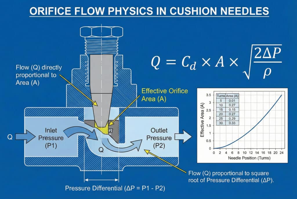
The Orifice Flow Equation

Turbulent flow through small orifices follows established fluid dynamics:

$$
Q = C_{d} \times A \times \sqrt{\frac{2 \Delta P}{\rho}}
$$

Kus:

• Q = Volumetric flow rate (m³/s or SCFM)
• Cd = Discharge coefficient (dimensionless, 0.6-0.8)
• A = Effective orifice area (m² or mm²)
• ΔP = Pressure differential (Pa or psi)
• ρ = Air density (kg/m³, approximately 1.2 at standard conditions)

Simplified for Pneumatic Applications:
$$
Q\;(\text{SCFM})
\approx 0.5 \times A\;(\text{mm}^{2}) \times \sqrt{\Delta P\;(\text{psi})}
$$

This reveals that doubling orifice area doubles flow, but doubling pressure only increases flow by 41% (√2 = 1.41).

Needle Position and Orifice Area

The needle valve geometry determines area vs. position relationship:

Typical Needle Valve Design:

• Tapered needle: 30-60° cone angle
• Seat diameter: 2-6mm depending on cylinder size
• Thread pitch: 0.5-1.0mm per turn
• Adjustment range: 10-20 turns from closed to fully open

Area vs. Turns Relationship:

Needle Position	Efektiivne ala	Flow Rate (at 400 psi ΔP)	Relative Flow
Closed + 0.5 turns	0.1 mm²	1,0 SCFM	1x (baastase)
Closed + 1 turn	0.3 mm²	3.0 SCFM	3x
Closed + 2 turns	0.8 mm²	8.0 SCFM	8x
Closed + 3 turns	1.5 mm²	15.0 SCFM	15x
Closed + 5 turns	3.0 mm²	30.0 SCFM	30x
Fully open (10+ turns)	5.0 mm²	50.0 SCFM	50x

Notice the non-linear relationship—early turns have much larger impact than later turns.

Pressure Differential Dynamics

Cushion chamber pressure varies throughout the deceleration stroke:

Pressure Profile During Cushioning:

1. Initial engagement: ΔP = 50-100 psi (low flow needed)
2. Mid-compression: ΔP = 200-400 psi (moderate flow)
3. Peak compression: ΔP = 400-800 psi (maximum flow)
4. Release phase: ΔP decreases as chamber expands

The square-root relationship means flow increases less than pressure:

• 100 psi ΔP → Baseline flow
• 400 psi ΔP → 2x baseline flow (not 4x)
• 900 psi ΔP → 3x baseline flow (not 9x)

Discharge Coefficient Variations

Cd depends on orifice geometry and flow conditions:

Factors Affecting Cd:

• Sharp-edged orifices: Cd = 0.60-0.65 (most needle valves)
• Rounded orifices: Cd = 0.70-0.80 (premium designs)
• Reynoldsi arv: Cd increases slightly at higher Re
• Saastumine: Particles reduce Cd by 10-30%

Bepto Premium Needle Valves:
We use precision-machined seats with 0.2mm radius edges, achieving Cd = 0.72-0.75 compared to 0.60-0.65 for standard sharp-edged designs. This provides 15-20% more flow at the same needle position, enabling finer adjustment control. 🎯

Temperatuuri ja tiheduse mõju

Air properties change with temperature:

Temperature Impact on Flow:

• Cold air (0°C): ρ = 1.29 kg/m³ → 3% higher flow resistance
• Standard (20°C): ρ = 1.20 kg/m³ → Baseline
• Hot air (60°C): ρ = 1.06 kg/m³ → 6% lower flow resistance

For most applications, temperature effects are minor (±5%), but extreme environments may require seasonal adjustment.

How Does Flow Regime Affect Cushioning Performance?

The transition between laminar and turbulent flow creates dramatically different cushioning behavior. 🌊

Flow regime determines cushioning characteristics: laminar flow (Reynolds number <2300) provides linear damping where force is proportional to velocity, while turbulent flow (Re >4000) creates square-law damping where force increases with velocity squared. Most cushion needles operate in turbulent regime during active cushioning (Re = 5000-20,000) but may transition to laminar during final settling (Re <2000), causing two-stage deceleration behavior. This regime transition explains why cushioning feels “soft” initially then “firms up” during final compression, and why adjustment sensitivity varies with operating speed.

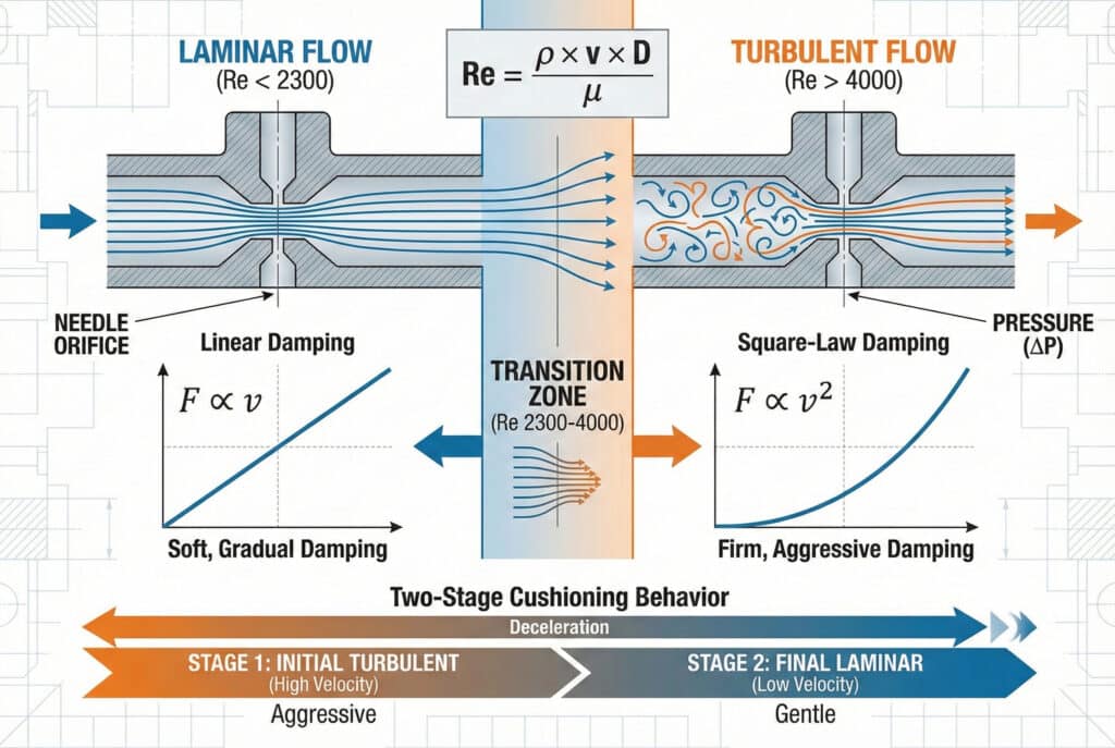
Reynolds Number and Flow Regime

Reynolds number determines flow behavior:

$$
Re = \frac{\rho \times v \times D}{\mu}
$$

Kus:

• ρ = Air density (1.2 kg/m³)
• v = Flow velocity (m/s)
• D = Orifice diameter (m)
• μ = Dünaamiline viskoossus⁴ (1.8 × 10⁻⁵ Pa·s for air)

Flow Regime Classification:

• Re < 2,300: Laminar flow (smooth, predictable)
• Re = 2,300-4,000: Transition zone (unstable)
• Re > 4,000: Turbulent flow (chaotic, energy-dissipating)

Typical Cushion Needle Values:

• Orifice diameter: 1-3mm
• Flow velocity: 50-200 m/s (sonic velocities possible)
• Reynolds number: 5,000-25,000 (strongly turbulent)

Laminar vs. Turbulent Damping Characteristics

Different flow regimes create different cushioning feel:

Iseloomulikud	Laminaarne voolu	Turbulentne voolu
Damping force	F ∝ v (linear)	F ∝ v² (square-law)
Low-speed behavior	Soft, gradual	Very soft, minimal
High-speed behavior	Mõõdukas	Firm, aggressive
Adjustment sensitivity	Pidev	Velocity-dependent
Rõhu kogunemine	Gradual, linear	Rapid, exponential
Energia hajutamine	Low efficiency	High efficiency
Typical Re range	500-2,000	5,000-25,000

Two-Stage Cushioning Behavior

Many cylinders exhibit regime transition during deceleration:

Stage 1 – Initial Deceleration (Turbulent):

• High velocity (1.0-2.0 m/s)
• High Reynolds number (10,000-20,000)
• Turbulent flow through needle orifice
• Aggressive damping force
• Rapid velocity reduction

Transition Zone:

• Velocity drops to 0.3-0.5 m/s
• Reynolds number decreases to 2,000-4,000
• Flow becomes unstable
• Damping characteristics change

Stage 2 – Final Settling (Laminar):

• Low velocity (<0.3 m/s)
• Low Reynolds number (<2,000)
• Laminar flow develops
• Softer damping force
• Slower final approach

This two-stage behavior is why properly adjusted cushioning feels “firm but smooth”—aggressive initial deceleration followed by gentle final positioning.

Velocity-Dependent Adjustment Sensitivity

Needle adjustment has different effects at different speeds:

Low-Speed Operation (0.5 m/s):

• May operate in laminar regime
• Linear damping: F ∝ v
• Needle adjustment creates proportional force change
• 1 turn adjustment → 30-50% force change

High-Speed Operation (2.0 m/s):

• Operates in turbulent regime
• Square-law damping: F ∝ v²
• Needle adjustment creates squared force change
• 1 turn adjustment → 60-120% force change

This explains Jennifer’s Oregon facility problem: At low speeds (0.8 m/s), her needle settings worked fine. At high speeds (1.8 m/s), the same settings created 3-4x more damping force than expected due to turbulent regime square-law behavior. 💡

Sonic Flow Conditions

At very high pressure differentials, flow becomes choked⁵:

Sonic (Choked) Flow:

• Occurs when ΔP > 0.5 × P_downstream
• Flow velocity reaches speed of sound (≈340 m/s)
• Further pressure increase doesn’t increase flow rate
• Flow rate becomes: Q = Cd × A × P_upstream / √T

Implications for Cushioning:

• Maximum flow rate is limited regardless of pressure
• Very small orifices may choke during peak compression
• Choked flow creates maximum damping force
• Needle adjustment less effective when choked

Typical Conditions for Choked Flow:

• Cushion pressure: >600 psi
• Exhaust pressure: <300 psi
• Pressure ratio: >2:1
• Common in: Small orifices (<0.5 mm²), high-speed cylinders

Why Does Needle Adjustment Sensitivity Vary Non-Linearly?

Understanding the geometric and fluid dynamic factors reveals why adjustment behavior seems unpredictable. 📐

Needle adjustment sensitivity varies non-linearly due to three factors: geometric area change (tapered needle creates exponential area increase with linear position change), flow regime transitions (moving from turbulent to laminar changes damping from square-law to linear), and pressure-dependent flow (higher pressures reduce relative impact of area changes due to square-root relationship). The first 2-3 turns from closed position typically control 60-80% of total flow range, while the final 5-7 turns provide only 20-40% additional flow, making initial adjustment critical and fine-tuning progressively less sensitive.

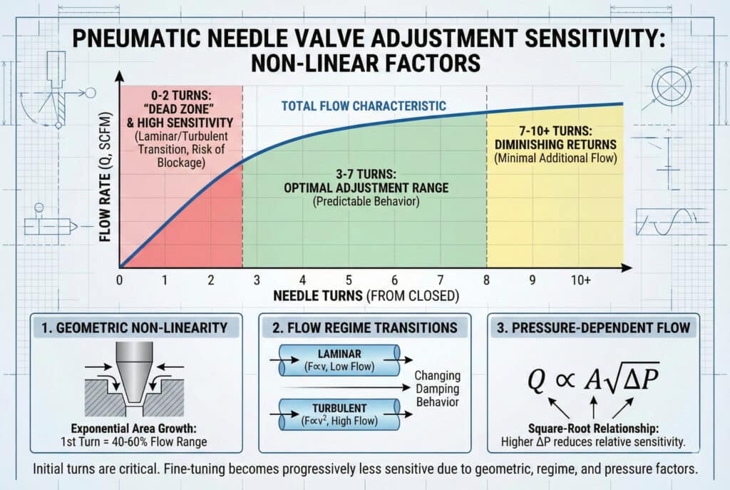
Geometric Non-Linearity

Tapered needle geometry creates exponential area growth:

Needle Valve Geometry:

• Cone angle: 30-60° typical
• Seat diameter: 3mm example
• Thread pitch: 0.8mm/turn example

Area Calculation:
For a 45° cone angle:

• 0.5 turns (0.4mm lift): A = π × 3mm × 0.4mm × sin(45°) = 2.7 mm²
• 1.0 turns (0.8mm lift): A = π × 3mm × 0.8mm × sin(45°) = 5.3 mm²
• 2.0 turns (1.6mm lift): A = π × 3mm × 1.6mm × sin(45°) = 10.7 mm²

Sensitivity Analysis:

Reguleerimisvahemik	Area Change	Flow Change	Tundlikkus
0 → 1 turn	0 → 5.3 mm²	0 → 53 SCFM	Väga kõrge
1 → 2 turns	5.3 → 10.7 mm²	53 → 107 SCFM	Kõrge
2 → 3 turns	10.7 → 16.0 mm²	107 → 160 SCFM	Mõõdukas
3 → 5 turns	16.0 → 26.7 mm²	160 → 267 SCFM	Madal
5 → 10 turns	26.7 → 53.3 mm²	267 → 533 SCFM	Väga madal

The first turn creates as much flow change as turns 5-10 combined!

The “Dead Zone” Near Closed Position

Very small orifices behave differently:

Closed to 0.5 Turns:

• Orifice area: 0.05-0.5 mm²
• Flow may be laminar (Re <2000)
• Contamination highly likely to block flow
• Adjustment extremely sensitive
• Often considered “unusable range”

Parim praktika:
Never operate closer than 1.5-2 turns from fully closed to avoid:

• Unpredictable laminar/turbulent transitions
• Contamination blockage risk
• Excessive adjustment sensitivity
• Potential complete flow blockage

Pressure-Dependent Sensitivity

Square-root relationship affects adjustment impact:

Low Pressure Differential (100 psi):

• Flow: Q = 0.5 × A × √100 = 5 × A
• Doubling area doubles flow
• High adjustment sensitivity

High Pressure Differential (400 psi):

• Flow: Q = 0.5 × A × √400 = 10 × A
• Doubling area doubles flow (same absolute sensitivity)
• But flow is already 2x higher, so relative sensitivity is lower

Practical Impact:
At high speeds (high ΔP), needle adjustment has less relative impact on cushioning behavior because baseline flow is already high. This explains why high-speed applications often require larger adjustments to achieve noticeable changes.

Optimal Adjustment Range

Most effective needle positions for controllable adjustment:

Recommended Operating Range:

• Minimum position: 2 turns from fully closed
• Optimal range: 3-7 turns from closed
• Maximum useful: 10 turns from closed
• Beyond 10 turns: Minimal additional effect

Why This Range:

• Below 2 turns: Too sensitive, contamination risk
• 3-7 turns: Good sensitivity, predictable behavior
• Above 10 turns: Diminishing returns, approaching “fully open”

Bepto Precision Needle Design

We’ve optimized needle geometry for better adjustment linearity:

Standard Needle (60° cone):

• Highly non-linear response
• First turn = 40% of total flow range
• Difficult to fine-tune

Bepto Progressive Needle (30° cone + stepped design):

• More linear response across adjustment range
• First turn = 15% of total flow range
• Easier fine-tuning and repeatability
• Available on premium cylinder models (+$35) 🎯

Jennifer’s Oregon facility benefited significantly from switching to our progressive needle design, which provided predictable adjustment across her 0.8-1.8 m/s speed range.

How Do You Optimize Needle Settings for Consistent Performance?

Systematic optimization methodology delivers predictable cushioning across operating conditions. 🔧

Optimize needle settings by calculating required flow rate using Q = V_chamber / t_deceleration (chamber volume divided by desired deceleration time), then determining needle position from flow equation Q = 0.5 × A × √ΔP, starting at mid-range (4-5 turns open) and adjusting in half-turn increments while measuring settling time and bounce. Target settling time of 0.2-0.3 seconds with less than 2mm overshoot. For variable-speed applications, optimize at maximum speed (worst case) then verify acceptable performance at minimum speed, accepting slight over-cushioning at low speeds rather than under-cushioning at high speeds.

Vooluhulga arvutamise meetod

Determine required flow based on cushion chamber volume:

Step 1: Calculate Chamber Volume

• Measure or obtain cushion chamber dimensions
• Example: 80mm bore, 25mm cushion stroke
• Volume = π × (40mm)² × 25mm = 125,664 mm³ = 125.7 cm³

Step 2: Determine Desired Deceleration Time

• Target: 0.15-0.25 seconds for most applications
• Example: 0.20 seconds

Step 3: Calculate Required Flow Rate

• Q = Volume / Time
• Q = 125.7 cm³ / 0.20s = 628.5 cm³/s
• Convert: 628.5 cm³/s × 0.00212 = 1.33 SCFM

Step 4: Estimate Pressure Differential

• Typical peak: 400-600 psi
• Use 500 psi for calculation

Step 5: Calculate Required Orifice Area

• Q = 0.5 × A × √ΔP
• 1.33 = 0.5 × A × √500
• A = 1.33 / (0.5 × 22.4) = 0.119 mm²

Step 6: Determine Needle Position

• Refer to valve calibration curve
• For typical valve: 0.119 mm² ≈ 2.5 turns from closed

Systematic Adjustment Procedure

Follow this step-by-step process:

Esialgne seadistamine:

1. Start with needle valve 4-5 turns open (mid-range)
2. Run cylinder at normal operating speed and load
3. Observe cushioning behavior

Adjustment Iterations:

Observed Behavior	Probleem	Kohandamine	Expected Result
Hard impact, no deceleration	Under-cushioned	Close 2 turns	Smoother stop
Bounce 5-15mm, oscillation	Over-cushioned	Open 2 turns	Reduced bounce
Slight bounce 2-5mm	Slightly over-cushioned	Open 1 turn	Minimal overshoot
Smooth but slow settling	Slightly over-cushioned	Open 0.5 turns	Kiirem settimine
Smooth, fast settling	Optimaalne	Ei ole muutusi	Maintain setting

Fine-Tuning:

• Make adjustments in 0.5-turn increments near optimal
• Test 5-10 cycles after each adjustment
• Document final settings for future reference

Variable Speed Optimization

For applications with speed variation:

Strategy 1: Worst-Case Optimization

• Optimize for maximum speed (highest kinetic energy)
• Accept slight over-cushioning at lower speeds
• Pros: Simple, safe, reliable
• Cons: Not optimal at all speeds

Strategy 2: Compromise Setting

• Optimize for average operating speed
• Acceptable performance across range
• Pros: Better average performance
• Cons: Not optimal at extremes

Strategy 3: Adjustable Shock Absorbers

• Use external absorbers with rotary dial adjustment
• Quick adjustment for different speeds
• Pros: Optimal at all speeds
• Cons: Higher cost ($150-300 per absorber)

Pressure Compensation Techniques

Account for system pressure variations:

Fixed Pressure Systems (±5 psi variation):

• Single needle setting adequate
• No compensation needed

Variable Pressure Systems (±15+ psi variation):

• Pressure variations affect cushioning significantly
• Options:
    1. Regulate pressure to cylinder (add pressure regulator)
    2. Use pressure-compensated shock absorbers
    3. Accept performance variation
    4. Optimize for minimum pressure (conservative)

Jennifer’s Oregon Facility Solution

We implemented comprehensive optimization:

Problem Analysis:

• Speed range: 0.8-1.8 m/s (2.25:1 variation)
• Load: 22kg constant
• Existing setting: 3 turns open
• Performance: Good at 0.8 m/s, violent at 1.8 m/s

Flow Calculations:

• Low speed KE: ½ × 22 × 0.8² = 7.0 J
• High speed KE: ½ × 22 × 1.8² = 35.6 J
• Energy ratio: 5.1:1 (explains the problem!)

Solution Implemented:

1. Replaced standard needles with Bepto progressive design
      – Better linearity across adjustment range
      – More predictable behavior

2. Optimized for high-speed operation
      – Needle setting: 5.5 turns open (vs. 3 previously)
      – High-speed performance: Smooth, 0.18s settling
      – Low-speed performance: Acceptable, 0.28s settling

3. Added external shock absorbers to 6 critical stations
      – Rotary dial adjustment for quick speed changes
      – Optimal performance at all speeds
      – Cost: $1,800 for 6 units

Results After Optimization:

• High-speed impacts: Eliminated
• Settling time consistency: ±0.05s across speed range
• Adjustment time for speed changes: <30 seconds
• Cycle time improvement: 18% (faster settling)
• Product damage: Reduced 94% (from 3.2% to 0.2%)
• Annual savings: $127,000 in reduced waste
• Investment payback: 2.1 weeks 💰

Bepto Optimization Support

We provide technical assistance for cushioning optimization:

Services Offered:

• Flow calculation worksheets
• Needle position recommendations
• On-site optimization support (select regions)
• Phone/video consultation
• Custom needle valve calibration

Optimization Packages:

• Basic: Calculation support and recommendations (Free)
• Standard: Phone consultation + custom calculations ($150)
• Premium: On-site optimization service ($800-1,500)

Kokkuvõte

Orifice flow dynamics in cushion needle valves follow predictable fluid mechanics principles—understanding the turbulent flow equation, geometric non-linearity, and flow regime transitions transforms seemingly mysterious adjustment behavior into systematic, optimizable performance. By calculating required flow rates, accounting for pressure differentials, and following methodical adjustment procedures, you can achieve consistent cushioning across varying speeds, loads, and operating conditions. At Bepto, we provide precision needle valves, technical calculation support, and optimization expertise to help you master cushioning performance in your pneumatic systems.

FAQs About Cushion Needle Flow Dynamics

1. Explore the branch of physics concerned with the mechanics of fluids (liquids, gases, and plasmas) and the forces on them. ↩

2. Learn about the dimensionless quantity used to predict flow patterns in different fluid flow situations. ↩

3. Understand the ratio of the actual discharge to the theoretical discharge for flow measurement devices. ↩

4. Read about the measure of a fluid’s internal resistance to flow and shear stress. ↩

5. Learn about the compressible flow effect where fluid velocity is limited by the speed of sound. ↩