How Valve Response Time Consistency Affects Machine Synchronization

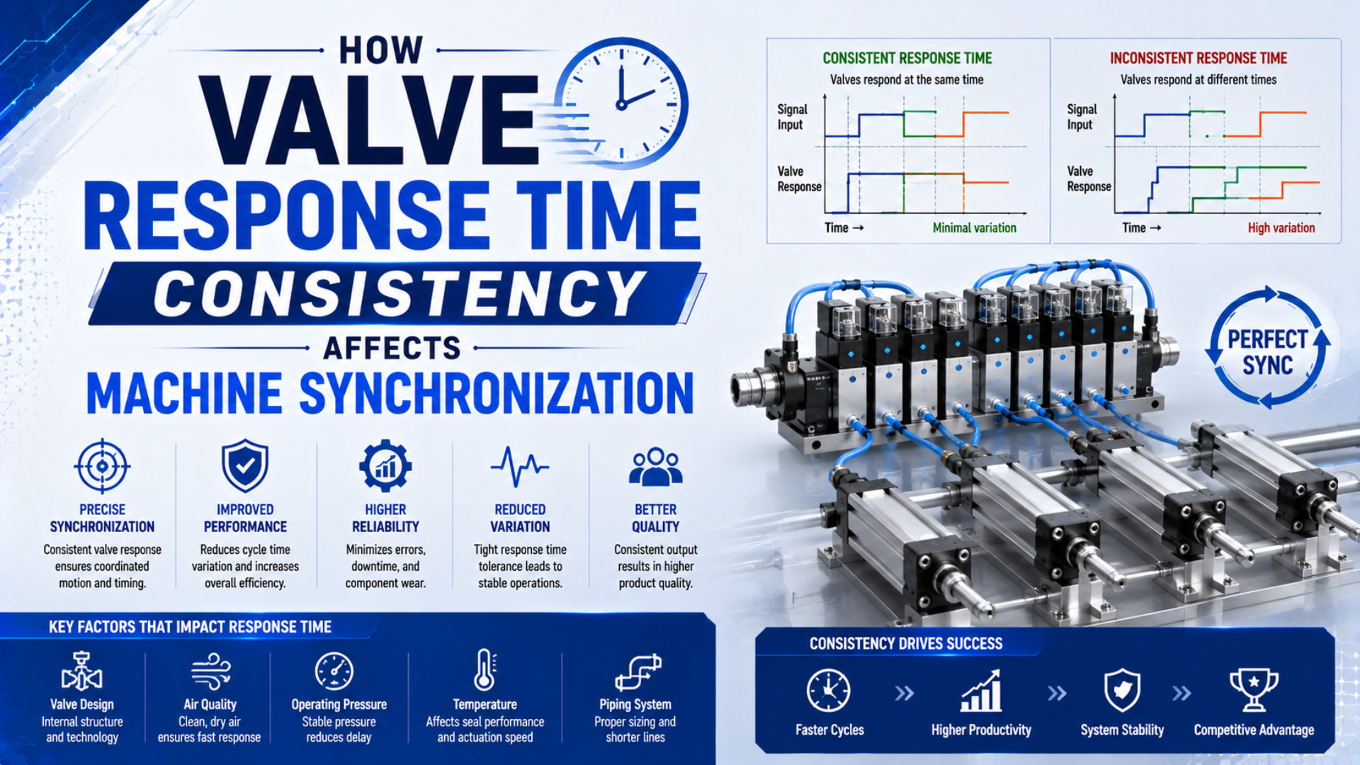
Valve response-time consistency affects synchronization through the difference between channels, not through one valve’s catalog speed alone. A stable delay can often be scheduled into the controller. Cycle-to-cycle jitter, thermal drift, and rare slow shifts change that difference unpredictably, so paired axes no longer reach their process events together.

There is no universal acceptable band such as ±5 ms or ±10 ms. Convert the machine’s allowable position or process-window mismatch into a timing limit, then test the complete command-to-event chain under representative operating conditions.

Key Takeaways

• Synchronization depends on relative timing skew between channels, not simply the fastest individual valve.
• Festo lists response as low as 2 ms and repetition accuracy around 0.2 ms for specific fast-switching valves; those are separate, model-specific specifications.
• A fixed offset can correct stable bias, but it cannot remove random jitter, outliers, or a changing pneumatic delay.

In this guide

• What does valve response-time consistency mean?
• How does timing skew become a synchronization error?
• The command-to-event delay chain
• Shared and channel-specific disturbances
• How should you build a synchronization acceptance test?
• What can software compensation fix?
• How do you diagnose lost synchronization?
• Valve response-time consistency FAQs

What Does Valve Response-Time Consistency Mean?

ISO 12238:2023 defines procedures for measuring the shifting time of electrically or pneumatically operated directional valves with two- or three-position functions. Its scope makes an important boundary clear: valve shifting time is a component measurement, while synchronized machine arrival also includes the air path, actuator, load, and sensor (ISO 12238:2023).

Valve response-time consistency is the stability of a defined command-to-valve event across repeated cycles and stated operating conditions. It cannot be evaluated until the start event, end event, pressure, voltage, temperature, and test arrangement are identified.

Use four different terms in specifications and test reports:

Term	Practical meaning	Question it answers
Latency	Delay from a defined start event to a defined end event	How late is the event on average?
Jitter	Cycle-to-cycle spread around the usual delay	How repeatable is the event?
Drift	A gradual change in the center of the timing distribution	Does warm-up, wear, or environment move the delay?
Outlier	A rare event much slower or faster than the normal population	Can an occasional shift break the process window?

A valve can be fast but inconsistent, or slower but highly repeatable. Festo’s fast-switching-valve literature, for example, publishes response down to 2 ms and repetition accuracy around 0.2 ms for specified MH-series products. Those figures demonstrate that response and repeatability are separate attributes; they do not establish a general pneumatic-valve limit (Festo Fast Switching Valves). Likewise, SMC lists a representative 10 ms response for one SY3000 single-solenoid configuration at 0.5 MPa and 20°C. That value belongs to the stated model and conditions, not to every SY valve or every machine installation (SMC SY Series).

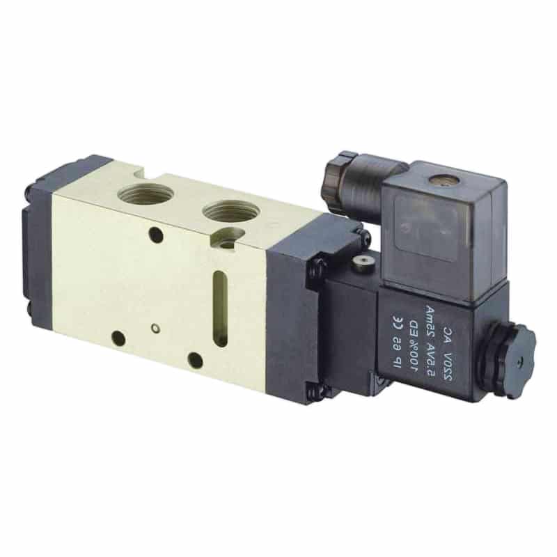
Two nominally similar directional valves can still develop different command-to-event delays because their drivers, pilot conditions, air paths, loads, and temperatures are not necessarily identical.

For synchronization work, the most useful performance object is not “Valve A response time.” It is the distribution of the paired difference between Axis A and Axis B under the same cycle conditions. That paired signal cancels some shared disturbances and exposes the mismatch that the machine actually experiences.

How Does Timing Skew Become a Synchronization Error?

A 10 ms timing difference has no fixed mechanical meaning. At a relative motion speed of 1 m/s, it corresponds to about 10 mm; at 0.05 m/s, it corresponds to about 0.5 mm. The same delay can therefore be harmless in one process and unacceptable in another.

Synchronization skew is the signed time difference between corresponding events on two channels measured from a common reference clock. It is the direct timing variable to compare with a machine-specific process window.

For cycle number $i$, define the relative synchronization skew as:

Here, $t_{A,i}$ and $t_{B,i}$ are the measured times in seconds from a common command reference to the selected events on axes A and B. A positive result means A occurred after B; a negative result means A occurred before B.

If both mechanisms are still moving near the critical event, a first-order position-mismatch estimate is:

Here, $\Delta x_i$ is the approximate mismatch in metres, and $v_{\mathrm{rel},i}$ is the relative speed in metres per second at the event. The approximation assumes speed is nearly constant across the short timing interval. It does not include acceleration, compliance, impact, sensor hysteresis, or controller scan effects.

Derive the initial timing allowance from the process window:

Here, $t_{\mathrm{allow}}$ is the timing allowance in seconds and $x_{\mathrm{allow}}$ is the permitted mismatch in metres. The engineering acceptance limit should also reserve margin for measurement uncertainty and other sources of machine variation. Do not use this simple relation as a safety calculation.

The cylinder response-time and dead-volume analysis explains why pressure arrival and piston motion remain different events. For flow-capacity decisions, use the separate guide to sizing a solenoid valve for a target stroke time.

The Command-to-Event Delay Chain

Texas Instruments’ DRV110 solenoid driver deliberately uses a current ramp, a peak-current interval, and a lower hold-current phase. That three-stage behavior illustrates why the electrical driver belongs inside the timing budget rather than being treated as an invisible part of the PLC output (Texas Instruments DRV110).

Command-to-event delay is the elapsed time from a declared electrical reference to a declared pneumatic, mechanical, or process event. Its value grows as the measurement boundary moves downstream.

The complete machine delay can include:

1. PLC task scheduling and output-module update.
2. Cable, connector, suppression circuit, and solenoid driver behavior.
3. Coil-current rise and magnetic-force buildup.
4. Armature, pilot stage, or main-spool movement.
5. Outlet-pressure rise or exhaust-pressure decay.
6. Manifold passage, fitting, tube, speed controller, and muffler effects.
7. Cylinder breakaway, acceleration, load motion, cushioning, and sensor switching.

If the coil edges differ, the pneumatic circuit has not yet been tested fairly. If the coil edges match but valve-outlet pressure differs, inspect the driver, coil, pilot stage, and valve. If outlet traces match but actuator-port traces separate, inspect manifold flow, tubes, fittings, flow controls, and exhaust. If both pressure traces match but sensor arrival differs, inspect mechanics, load, cushioning, alignment, and sensing.

This downstream comparison extends the measurement method in the complete guide to solenoid-valve response-time measurement without repeating its generic bench procedure.

Shared and Channel-Specific Disturbances

SMC warns that continuous energization raises valve temperature because of coil heat and can affect performance. On synchronized channels, the effect may remain mostly common-mode if duty and cooling are alike, or become differential when one coil stays energized longer, sits beside a heat source, or has different ventilation (SMC Installation and Maintenance Manual).

Disturbance	Usually shared or channel-specific?	What to compare
PLC task or network update	Shared unless outputs use different modules or tasks	Command edges on the same timebase
Common supply-pressure sag	Shared, but manifold geometry can distribute it unevenly	Manifold inlet and both working ports during simultaneous demand
Coil temperature and duty cycle	Often channel-specific	Coil current, surface temperature, energization pattern
Tube length and internal diameter	Channel-specific	Installed route, ID, fittings, downstream volume
Valve friction or contamination	Channel-specific	Valve-outlet pressure edge and repeat distribution
Exhaust muffler restriction	Channel-specific unless a common exhaust is used	Exhaust back pressure and decay trace
Load, seal friction, and alignment	Channel-specific	Actuator-port pressure versus sensor arrival
Ambient temperature	Shared at cabinet level, potentially different near the machine	Temperature at each valve and actuator

Common-mode delay moves both axes later by a similar amount and may leave relative skew nearly unchanged. Differential delay separates the axes and directly harms synchronization. A shared disturbance can still become differential when the manifold, branches, duty cycles, or loads are asymmetric. Test shared and differential behavior separately. First fire each axis alone, then fire both together. If the pair becomes less synchronized only during simultaneous demand, the dominant problem may be shared supply capacity or manifold distribution rather than either valve’s standalone response.

How Should You Build a Synchronization Acceptance Test?

NIST treats the process center and process variability as separate control-chart questions: an X-bar chart monitors the mean, while R or S charts monitor spread. That same distinction suits valve timing because a stable average can conceal growing variation, and low variation can coexist with a biased channel (NIST Control Charts).

Write the acceptance definition before collecting data:

Test field	Required decision
Start event	PLC command, output-module voltage edge, or coil-current threshold
End event	Valve-outlet pressure, actuator-port pressure, position switch, encoder position, or process sensor
Synchronization metric	Paired Axis A minus Axis B event time
Conditions	Supply pressure, voltage, temperature, load, tube route, flow settings, and exhaust state
Operating states	Cold start, thermal steady state, normal cycle rate, and simultaneous consumers
Summary	Count, minimum, maximum, mean, spread, percentiles, and outliers
Pass-fail rule	Machine-derived skew window and any separate absolute-delay limit
Instrumentation	Sensor range, accuracy, bandwidth, sample rate, trigger, and common clock

Measure the event the process depends on. Valve-outlet pressure is suitable for component diagnosis; cylinder arrival is suitable when end-position coordination matters; an encoder or process sensor is better when synchronization is required in mid-stroke. Do not substitute one boundary for another without relabeling the result. The sampling interval and sensor bandwidth must also resolve the limit with useful margin. A logger that updates every 10 ms cannot characterize a few-millisecond distribution. Record raw paired traces, not only an average exported by the PLC.

Use cold and stabilized tests because coil temperature, lubrication, seal friction, and air temperature can change during operation. Also repeat the test while other consumers create realistic pressure demand. No single cycle count is universally sufficient; choose enough observations to expose warm-up, ordinary variation, and rare events at the risk level of the application.

For coil-specific influences, see how coil inductance affects solenoid response time and the AC-versus-DC coil response comparison.

What Can Software Compensation Fix?

The DRV110 peak interval is set independently from its lower hold-current phase, showing that control electronics can intentionally shape solenoid behavior. Machine software can likewise schedule a stable channel offset, but neither method proves that the pneumatic output remains repeatable across pressure, temperature, load, and wear (Texas Instruments DRV110).

Use compensation according to the observed error type:

Observed timing behavior	Appropriate response	Limit
Stable channel bias	Apply a verified command offset	Revalidate after component or process changes
Slow, measurable drift	Consider bounded adaptive correction	Requires reliable feedback and fault limits
Random jitter	Diagnose driver, valve, air path, load, and sensor	A fixed offset cannot reduce spread
Rare extreme outlier	Find the physical or electrical fault and add process interlocks	An average-based correction can hide the event
Pressure-dependent delay	Stabilize supply or schedule only within a validated pressure model	Compensation cannot restore missing flow capacity

Never use two closed-center pneumatic valves and matching command times as proof of safety-rated load holding. Compressed air, leakage, valve state, trapped pressure, mechanics, and stored energy require a machine risk assessment and an appropriate safety architecture. A cascaded sequence may intentionally wait for confirmed completion rather than demand simultaneous open-loop motion; the pneumatic cascade-circuit design guide explains that event-driven alternative. Compensate the smallest stable boundary. If Axis A is always late at the coil edge, correct the command path. If coil edges match but pressure edges differ, correcting the PLC can mask a valve or air-path fault. The measurement boundary tells you whether compensation is control logic or concealment.

How Do You Diagnose Lost Synchronization?

ISO 12238:2023 applies to valve shifting time, so a valve-level trace is the right isolation step only after both channels share a verified electrical reference. If the final machine event is late but the valve-outlet pressure edges match, replacing the valve is unlikely to address the measured delay (ISO 12238:2023).

Use a boundary-by-boundary comparison:

1. Verify the reference. Capture both PLC or output-module command edges on one timebase.
2. Capture coil behavior. Compare voltage and current at each valve connector during the real cycle.
3. Measure valve output. Compare pressure rise and decay at both working ports.
4. Move downstream. Compare actuator-port pressure to reveal tube, fitting, flow-control, or exhaust differences.
5. Compare mechanical events. Capture position, speed, load, cushion entry, and sensor switching.
6. Change one condition. Swap electrical channels, valves, tubes, or loads one at a time when the machine permits.
7. Repeat hot and cold. Determine whether the center, spread, or outlier rate changes with duty.

Finding	Likely investigation area
Command edges differ	PLC task, network, output module, wiring logic
Command matches; coil current differs	Voltage drop, connector, driver, suppression, coil temperature
Coil current matches; valve pressure differs	Pilot pressure, spool friction, contamination, valve construction
Valve output matches; actuator-port pressure differs	Manifold, tube, fitting, flow control, muffler, leak
Port pressure matches; position differs	Load, alignment, seal friction, cushion, mechanism
Position matches; sensor event differs	Sensor mounting, hysteresis, wiring, input filtering

When the trace points to a channel-specific valve fault, use the solenoid-valve troubleshooting workflow before replacement. If the mismatch appears only at higher cycle rates, check flow capacity, exhaust restriction, pressure recovery, and thermal state before choosing a nominally faster valve.

About the author: Eric Zhou covers pneumatic control-system architecture for Bepto. Learn more on About Bepto or contact our engineering team to review an application-specific timing budget.

Valve Response-Time Consistency FAQs

Festo’s separate figures for response down to 2 ms and repetition accuracy around 0.2 ms summarize the central lesson: speed and consistency are not interchangeable specifications. The answers below therefore avoid a universal millisecond threshold and keep component response, installed pneumatic response, and machine arrival as distinct measurement boundaries (Festo Fast Switching Valves).

Is a faster valve always better for synchronization?

No. A faster valve can shorten average delay, but synchronization depends on the difference and spread between channels. A slightly slower, repeatable pair may be easier to coordinate than a fast pair with unstable jitter, provided both valves still meet the machine’s absolute cycle-time requirement.

What response-time variation is acceptable?

Acceptable variation is the machine-derived limit that keeps relative position or the process event inside its permitted window under validated conditions. Convert the allowable mismatch and relative speed into an initial timing budget, then reserve margin for measurement uncertainty and other sources of variation. There is no universal ±5 ms or ±10 ms rule.

Can PLC software compensate valve timing differences?

PLC software can compensate a stable, measured channel bias by advancing or delaying one command. It cannot remove random jitter, rare outliers, pressure starvation, or changing mechanical delay. Revalidate the offset after valve, driver, tubing, load, temperature, or cycle-rate changes.

Should valve response or cylinder arrival be measured?

Measure valve-outlet pressure to qualify or diagnose the valve. Measure actuator-port pressure to include the installed air path. Measure cylinder position or the process sensor when machine synchronization is the requirement. Using several boundaries on the same timebase reveals where the channels begin to separate.

Can two nominally identical valves respond differently?

Yes. Nominally identical valves can experience different driver voltage, coil temperature, pilot pressure, friction, contamination, tube volume, exhaust restriction, load, and sensor behavior. Compare paired traces under the installed conditions before deciding whether the difference belongs to the valves themselves.

Sources

• ISO 12238:2023, directional-control-valve shifting-time measurement scope and test procedures. Retrieved 2026-07-22.
• Festo Fast Switching Valves, model-specific response and repetition-accuracy examples for MH-series products. Retrieved 2026-07-22.
• SMC SY Series, representative response-time conditions for a specified SY3000 configuration. Retrieved 2026-07-22.
• Texas Instruments DRV110, peak-and-hold solenoid-current control phases. Retrieved 2026-07-22.
• NIST Control Charts, separate monitoring of process center and variability. Retrieved 2026-07-22.
• SMC Installation and Maintenance Manual, continuous-energization temperature caution. Retrieved 2026-07-22.