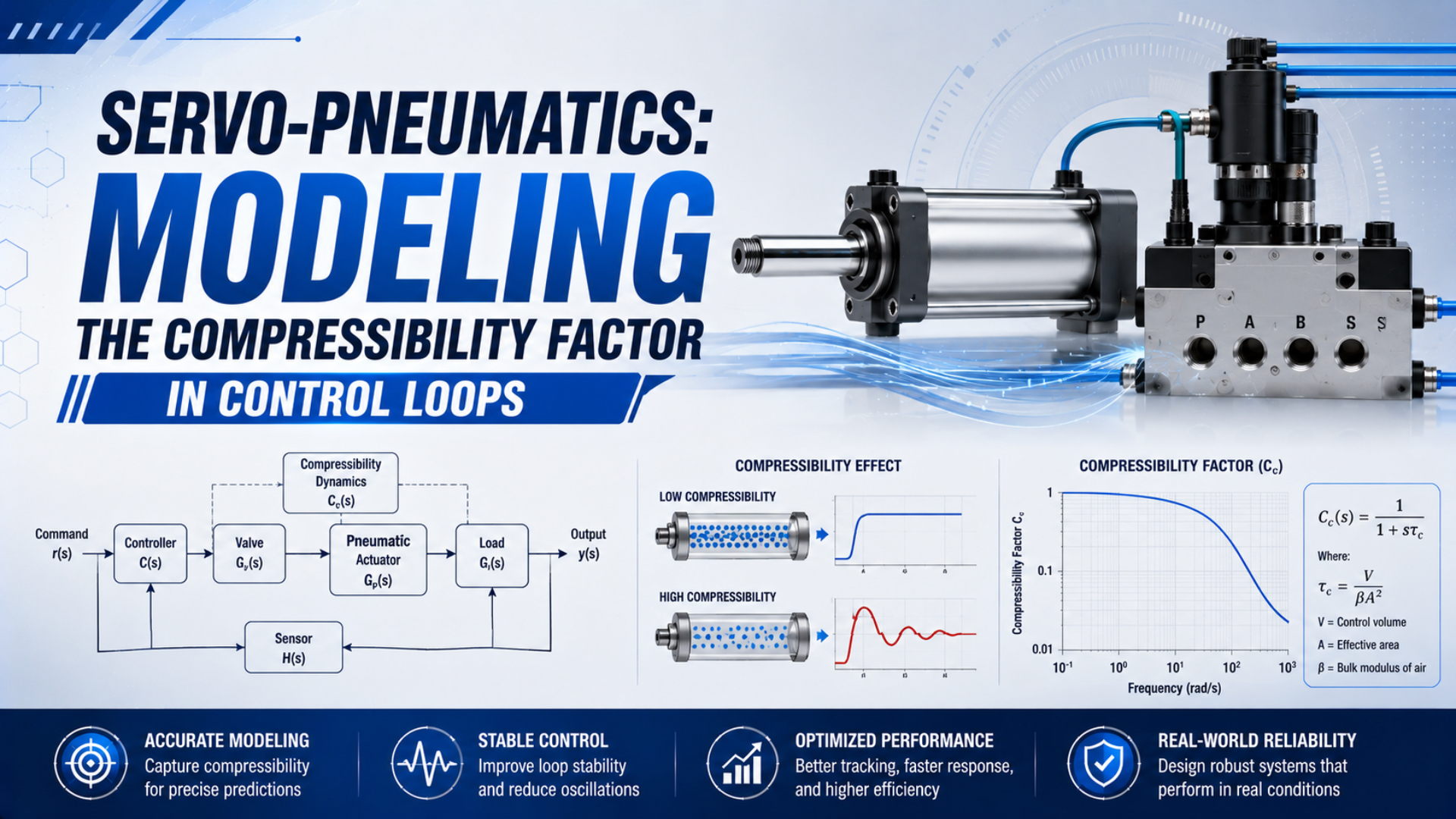
Servo-Pneumatics: Modeling the Compressibility Factor in Control Loops

Servo-pneumatic compressibility modeling does not treat “compressibility” as one adjustable constant. It separates the gas equation of state, the thermal-process assumption, the two changing chamber volumes, valve mass flow, piston force, friction, and moving mass. The result is a nonlinear plant that can be identified and validated before a controller is trusted.

This distinction matters because a servo-pneumatic positioning system contains at least three functional elements: an actuator with displacement feedback, a proportional directional valve, and a position controller (Festo, accessed 2026-07-23). A cylinder formula alone cannot predict the behavior of that complete loop.

Key Takeaways

• Model at least four core states: position, velocity, and two absolute chamber pressures.
• Use ISO 6358 data or measured valve maps instead of port size as a flow model.
• Linearize at defined operating points, then validate pressure and motion together before scheduling controller gains.

What Does Compressibility Factor Actually Mean?

NIST defines the dimensionless compressibility factor $Z$ as the correction for air non-ideality in a real-gas equation, not as cylinder stiffness or a controller gain (NIST, accessed 2026-07-23). Three different quantities must therefore stay separate in a servo-pneumatic model: $Z$, the process exponent, and mechanical air-spring stiffness.

For a mass-based real-gas model, write:

Units and reference states matter.

Here, $p$ is absolute pressure in pascals, $V$ is gas volume in cubic meters, $m$ is air mass in kilograms, $R$ is the specific gas constant for air, and $T$ is absolute temperature in kelvins. Setting $Z = 1$ gives the ideal-gas approximation. Whether that approximation is adequate depends on the required model accuracy, pressure, temperature, and humidity range. Compressibility factor is the real-gas correction described above. The polytropic exponent represents the assumed thermal path during compression or expansion. It answers a different question:

The exponent $n$ represents the assumed heat-transfer behavior over the modeled event, while $C$ is constant for that idealized process. It is not interchangeable with $Z$. A fast motion may approach an adiabatic assumption; a slow event with substantial heat exchange may behave closer to isothermal. The selected value must be documented and checked against measured pressure.

Pneumatic stiffness is a local force-versus-displacement result. For two trapped chambers, a useful small-signal approximation is:

The chamber pressures $p_1$ and $p_2$ must be absolute. Areas $A_1$ and $A_2$ are the effective piston areas, and volumes $V_1$ and $V_2$ include ports, fittings, tubing, and valve-side cavities trapped by the relevant valve state. This equation describes one operating point, not the complete moving-axis dynamics. For the physical meaning of this stiffness term and its change along the stroke, see the separate guide to air compressibility in cylinder control. The present article starts where that explanation ends: building a control model that can predict measured pressure and motion.

What Is the Minimum Nonlinear Plant Model?

Richer and Hurmuzlu validated a detailed pneumatic-actuator model on two cylinder types and multiple connecting-tube lengths, while accounting for nonlinear valve flow, chamber compressibility, leakage, inactive volume, and pneumatic-line effects (ASME, 2000). A practical first model can be smaller, but it cannot omit both chamber pressures.

Both pressure states are essential.

Choose a state vector that makes the stored pneumatic energy visible:

Position is $x$, velocity is $\dot{x}$, and $p_1$ and $p_2$ are absolute chamber pressures. Add valve-spool position, line states, temperature states, or friction states only when measurements show that the four-state model cannot reproduce the required behavior.

The two chamber volumes change in opposite directions:

$V_{10}$ and $V_{20}$ are the effective end volumes at the selected position origin, including clearance and connected dead volume. $L$ is usable stroke. Sign conventions can be reversed, but they must remain consistent in volume, pressure, force, and sensor equations.

Under a simplified ideal-gas, lumped-temperature, polytropic model, each chamber can be represented by:

$\dot{m}_i$ is signed net mass flow into chamber $i$. This equation is a modeling choice, not a universal law for every transient. If heat transfer, leakage, or temperature change creates unacceptable residual error, the energy model must be expanded instead of hiding the mismatch inside a controller gain.

The pneumatic force and moving-load equation are:

$M_{\mathrm{eq}}$ is the reflected moving mass. The remaining terms represent seal and guide friction, applied load, gravity where relevant, and mechanism forces. Rodless cylinders may have equal nominal pressure areas, but carriage friction, sealing bands, guidance, and external mechanics still make the two motion directions different.

In our experience, model order should follow observable error. Start with four states and measured valve maps. Add a state only when a repeated residual has a physical explanation, such as valve delay, line filling, thermal lag, or dynamic friction. A larger model with unidentified parameters can fit commissioning data yet predict new payloads worse.

How Should Valve Mass Flow Be Represented?

ISO 6358-1 defines a steady-state test method for compressible-fluid components with fixed or variable flow paths, but excludes cylinders, accumulators, regulators with internal feedback, and components with unstable coefficients (ISO, confirmed 2026). Use its valve data inside the plant model without treating the standard as a dynamic cylinder test.

Represent each metering edge as a signed function:

The valve command is $u$, upstream absolute pressure is $p_u$, downstream absolute pressure is $p_d$, and upstream temperature is $T_u$. The function must distinguish supply-to-chamber and chamber-to-exhaust flow, including choked and subsonic regions. A single nominal flow value does not define this surface.

Preferred inputs, in descending order, are:

1. A measured command-pressure-flow map for the exact valve and drive electronics.
2. Manufacturer curves with stated supply, downstream pressure, temperature, and command conditions.
3. ISO 6358 sonic conductance and critical pressure-ratio data for a compatible model.
4. A discharge-coefficient model whose geometry and assumptions have been validated.

Port size is not a flow model.

Neither is a catalog flow value measured under an unstated pressure convention. If the controller operates near valve deadband or saturation, identify those regions explicitly. Otherwise, the pressure model may look correct while the control input is wrong. Valve-to-cylinder tubing also belongs in the model boundary. Short lines reduce controlled volume, while small inside diameter can restrict mass flow. The related proportional-valve selection guide covers hardware sizing; this model should use the selected valve’s actual characteristic rather than a generic “servo valve” constant.

Linearization Around a Defined Operating Point

A 2004 servo-pneumatic study developed two local model structures, one black-box and one grey-box with pressure-difference and friction information, then scheduled state-feedback controllers across operating regions (Control Engineering Practice, 2004). The lesson is not a universal gain formula: every linear model belongs to a stated equilibrium and scheduling variable.

Local means local.

Write the nonlinear plant as $\dot{\mathbf{x}}_s = \mathbf{f}(\mathbf{x}_s,u)$ and choose an operating point $(\bar{\mathbf{x}}_s,\bar{u})$ that satisfies the equilibrium conditions. The local perturbation model is:

The matrices are Jacobians evaluated at the chosen operating point. Record piston position, payload, supply pressure, chamber pressures, valve bias, temperature assumption, and motion direction with every set. A transfer function with no operating point is incomplete because the chamber volumes and valve pressure ratios move as the axis travels.

The air-stiffness estimate can help interpret one pair of poles:

$\omega_n$ is an undamped local natural frequency in radians per second. It is not automatically the closed-loop bandwidth. Valve dynamics, damping, delay, feedback filters, saturation, friction, and unmodeled structure can shift the measured response. Use the separate natural-frequency calculation guide when resonance, rather than controller synthesis, is the primary question.

A gain schedule should interpolate verified controllers, not scale one proportional gain by chamber volume. Check every scheduled plant and the transitions between them. Position may be one scheduling variable, but payload, pressure, direction, and valve operating region can be equally important if they change during production.

Which Parameters Must Be Identified on the Machine?

A 2017 experimental methodology found that identifying dead volume improved model agreement for three measured outputs: chamber pressure, piston velocity, and piston position (Simulation Modelling Practice and Theory, 2017). That result makes dead volume a measured parameter, not a convenient value adjusted until one position trace looks right.

Separate parameters by how they can be obtained:

Parameter group	Starting source	Identification test	Validation signal
Bore, effective areas, stroke	Drawing and datasheet	Dimensional check	End positions and force balance
Chamber and connected dead volumes	CAD and tube-volume calculation	Isolated pressure-volume test	Both chamber-pressure traces
Valve flow surface	Manufacturer data	Controlled pressure-flow mapping	Pressure rise and exhaust decay
Valve deadband and delay	Electronics and valve datasheet	Small command sweeps and steps	Command-to-pressure onset
Moving mass and external load	Mass and mechanism calculation	Known-load motion test	Acceleration and force residual
Friction	Initial seal and guide data	Bidirectional low-speed and breakaway tests	Pressure-force residual versus velocity
Leakage	Component limits	Isolated pressure-hold test	Pressure decay with fixed volume
Thermal behavior	Assumed process model	Repeated slow and fast cycles	Pressure residual versus dwell and temperature

Do not identify all parameters from one position step. Several parameter combinations can produce similar motion while predicting the chamber pressures incorrectly. Use independent tests wherever possible, then reserve a separate dataset for validation. If the same data tunes and proves the model, overfitting can pass unnoticed. The measurement time base also matters. Record valve command, valve feedback if available, supply pressure at the valve, both cylinder-port pressures, position, payload, and timestamps synchronously. A static regulator gauge cannot show a pressure collapse during acceleration; the guide to air-pressure fluctuations explains that supply-side test. Position alone cannot separate flow restriction from breakaway friction.

How Does the Model Change Controller Design?

Festo describes three required elements in a servo-pneumatic positioning system, while the 2004 gain-scheduling study used local models plus state feedback rather than a universal PID multiplier (Festo, accessed 2026-07-23; Schulte and Hahn, 2004). Controller choice should follow measured plant variation and available feedback.

Observed plant behavior	Reasonable starting architecture	Required proof
One operating region, mild nonlinearity	Fixed-gain position or state controller	Stability and settling across normal load and pressure
Repeatable position-dependent dynamics	Gain-scheduled controller	Stability at every local plant and during interpolation
Tracking error dominated by known trajectory force	Model-based feedforward plus feedback	Inverse valve map, saturation handling, payload sensitivity
Chamber-pressure dynamics limit disturbance rejection	Pressure feedback inside the motion loop	Sensor bandwidth, noise, loop separation, fail behavior
Strong uncertainty or changing friction/load	Adaptive, uncertainty-aware, or nonlinear strategy	Bounded parameters, stability argument, worst-case tests

Feedforward begins with force balance, not a direct valve-command equation. The desired pressure force can be estimated as:

The required pair of chamber pressures must then respect supply pressure, exhaust pressure, force direction, and pressure limits. Converting those pressure targets into valve command requires the inverse valve-flow model and the chamber state. Dividing force by pressure difference and area does not produce a dimensionless valve command.

Do not copy a sampling rate from another machine. Select the controller period from the measured valve, pressure, sensor, computation, and mechanical dynamics, then preserve margin for filtering and delay. The safe commissioning sequence is conservative limits, verified signal polarity, open-loop characterization, one closed loop at a time, and finally the full payload and supply envelope.

For a broader hardware and commissioning overview, see the servo-controlled pneumatic positioning guide. Keep its component-selection task separate from the parameter-estimation task described here.

A Validation Workflow That Exposes the Wrong Model

The validated ASME model compared predictions on two cylinder types and different tube lengths, not just the dataset used for identification (Richer and Hurmuzlu, 2000). Your acceptance test should likewise include conditions that were withheld from fitting: another position, payload, direction, pressure, trajectory, or tube configuration.

Run validation in layers:

1. Static geometry and force: confirm areas, volumes, sign conventions, gravity, and equilibrium pressures.
2. Valve and chamber tests: compare measured and predicted pressure rise, pressure decay, deadband, and delay with fixed volume where practical.
3. Low-speed motion: expose breakaway friction, hysteresis, guide drag, and direction-dependent residuals.
4. Dynamic trajectories: compare command, both pressures, position, velocity, and acceleration under withheld operating conditions.
5. Closed-loop tests: verify settling, overshoot, steady error, saturation, disturbance response, and safe-state behavior at the process datum.

Residuals are evidence.

Inspect residual shape, not only one average error. A pressure residual that grows with dwell suggests thermal mismatch or leakage. A motion residual that changes sign with direction points toward friction or load modeling. A delay shared by both pressure traces may belong to the valve or acquisition chain. High-frequency position error with clean pressures can indicate sensor or mechanical dynamics outside the pneumatic model.

Validation should answer a decision question: is the model accurate enough for component selection, feedforward, gain scheduling, fault detection, or safety-related monitoring? Those uses require different error bounds. A model that estimates stroke time may still be inadequate for pressure-state feedback, and a good nominal model does not prove behavior after sensor, valve, or supply failure.

Before production release, define how stored pneumatic energy is isolated, how vertical or suspended loads are supported, what happens after loss of command or feedback, and how restart is authorized. Control performance never replaces the machine risk assessment.

Servo-Pneumatic Modeling FAQs

ISO 6358-1 covers steady-state component flow testing, while the validated nonlinear model cited above used two cylinder types and several tube configurations. These four questions address the boundaries most likely to corrupt a control model: gas terminology, pressure reference, operating-point coverage, and synchronized measurements (ISO, 2013; ASME, 2000).

Is compressibility factor Z the same as pneumatic stiffness?

No. $Z$ corrects the real-gas equation for non-ideal behavior. Pneumatic stiffness is a local force-displacement relationship derived from chamber pressure, effective piston area, trapped volume, and the assumed thermal process. A controller may use both concepts, but substituting one for the other produces the wrong units and the wrong physical interpretation.

Should the model use gauge pressure or absolute pressure?

Use absolute pressure in gas-state, density, pressure-ratio, mass-flow, stiffness, and temperature relationships. Gauge pressure can remain useful for operator displays and force calculations when atmospheric effects are handled consistently. Record the atmospheric reference and never insert a gauge value directly into an ideal-gas or polytropic equation.

Can one linear model cover the full cylinder stroke?

Only if validation shows that plant variation remains acceptable for the required performance. Chamber volumes, valve pressure ratios, friction, payload, and direction can change the local dynamics. For a wider envelope, identify several operating points and verify each controller plus the interpolation between them instead of assuming position-only gain scaling.

What signals should be recorded during model validation?

Record valve command, valve feedback when available, valve-inlet supply pressure, both cylinder-port pressures, position, payload condition, and synchronized timestamps. Derive velocity and acceleration with documented filtering. Add temperature, force, or flow when residuals indicate those states matter. Validate at the process datum, not only at the actuator’s internal sensor.

Sources and technical references

• NIST: Calculation of Compressibility Factor for Air, accessed 2026-07-23.
• ISO 6358-1: Determination of Flow-Rate Characteristics Using Compressible Fluids, accessed 2026-07-23.
• Richer and Hurmuzlu: A High Performance Pneumatic Force Actuator System, Part I, accessed 2026-07-23.
• Schulte and Hahn: Fuzzy State Feedback Gain Scheduling Control of Servo-Pneumatic Actuators, accessed 2026-07-23.
• Improved Nonlinear Modelling and Identification of a Servo-Pneumatic Actuating System, accessed 2026-07-23.
• Festo: Servo-Pneumatic Positioning Systems, accessed 2026-07-23.