The Physics of Air Hammer in Pneumatic Valve and Piping Systems

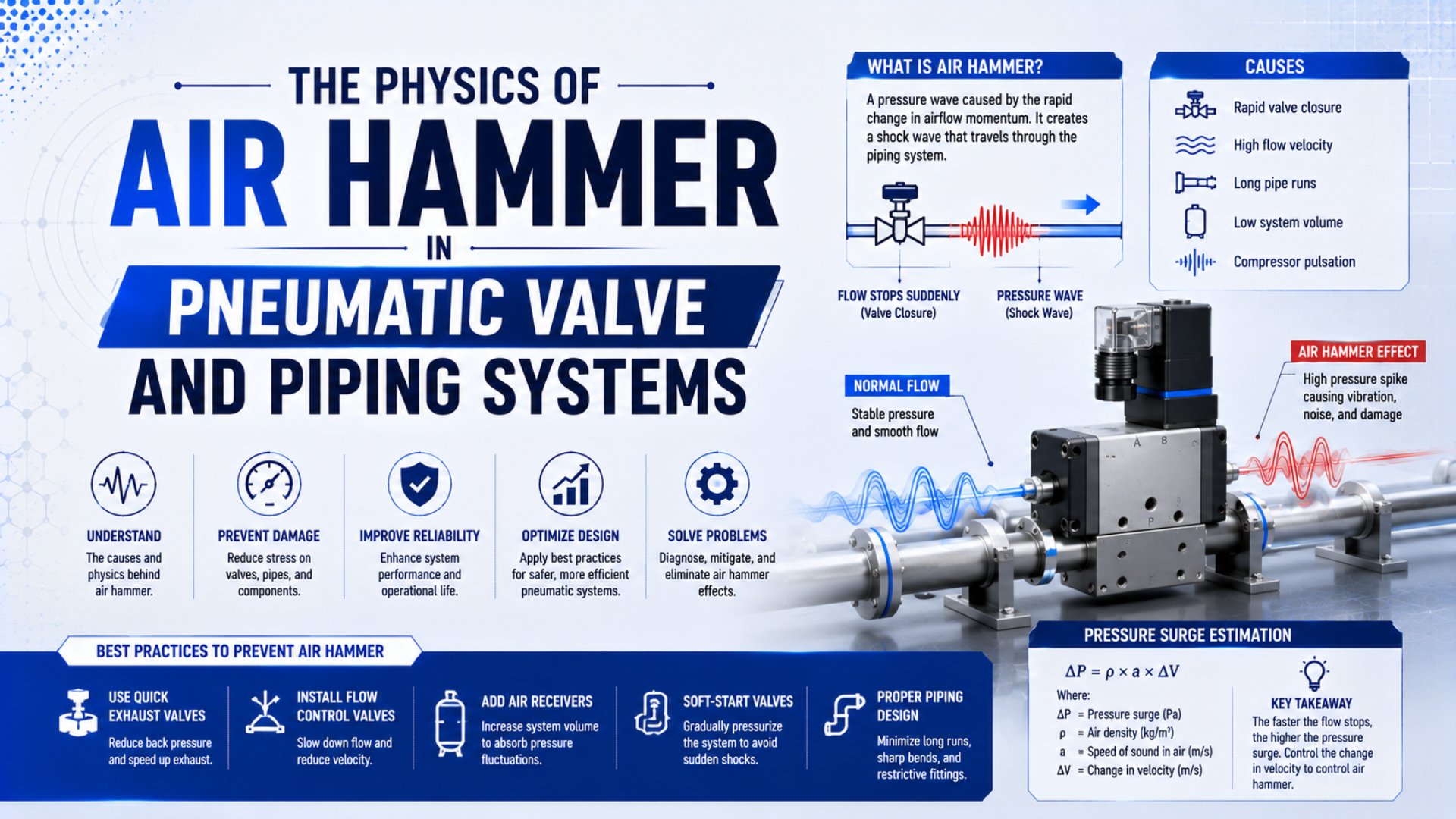
Air hammer in a pneumatic system is a short-lived pressure disturbance produced when a valve event, flow change, or volume connection changes the state of compressed gas faster than the piping network can settle. The disturbance travels as a compressible pressure wave, reflects at valves, branches, reservoirs, and closed volumes, and may load components dynamically. Its peak cannot be predicted safely by applying a universal multiplier to normal pressure.

That definition matters because “air hammer” is often used for several different faults. A bang at a machine may come from a dry-gas pressure transient, restricted exhaust, a cylinder striking its end cap, or condensate moving through a pipe. This article stays with one narrow subject: the physics and measurement of dry-gas transients associated with pneumatic valves and piping. For distribution moisture and restart problems, use the separate guide to water hammer in compressed-air systems.

Key Takeaways

• Near 20°C, a small disturbance in ideal dry air travels at approximately 343 m/s (NASA Glenn).
• Compare valve-event time with ${2L/a}$ for screening, not peak prediction.
• Liquid Joukowsky math is not a universal compressed-air formula.
• Use absolute state variables and synchronized dynamic measurements before choosing a remedy.

What Is Air Hammer in a Pneumatic System?

Pneumatic air hammer is a transient gas-flow event, not a steady pressure-drop problem. A rapid valve closure is one possible trigger, but rapid opening, check-valve movement, connection of unequal-pressure volumes, regulator response, and abrupt demand changes can also launch pressure and velocity disturbances (Rao and Eswaran, 1993).

The gas is compressible, so pressure, density, temperature, and velocity can all change while the disturbance moves. That makes the problem different from calculating pressure loss through a valve at constant operating conditions. ISO 6358-1 explicitly addresses steady-state flow testing of pneumatic components, while ISO 6358-3 estimates steady-state flow characteristics of connected components and piping (ISO 6358-1, 2013; ISO 6358-3, 2014). Sonic conductance and critical pressure ratio are valuable for sizing flow capacity, but they do not, by themselves, predict a transient pressure history.

Use more precise fault names during diagnosis:

Observed event	Likely physical problem	First evidence to collect
sharp pressure excursion immediately after a valve changes state	local compressible-gas transient	upstream and downstream dynamic pressure plus valve command/state
pressure sag while multiple consumers operate	steady or slowly varying supply restriction	pressure and flow across the distribution path
bang at cylinder end of stroke	moving mass and cushioning problem	piston speed, load energy, cushion and exhaust settings
bang after wet-air symptoms	condensate slug or liquid impact	drain status, low points, dew point and pipe temperature
movement during machine repressurization	uncontrolled filling and actuator force imbalance	downstream pressure rise and actuator position

The first event is more diagnostic than the loudest location. Frames, panels, and poorly supported pipes can radiate a pressure event that started elsewhere. In our experience, time-aligning the valve signal and pressure trace is the quickest way to challenge a false source location. Add a sound or acceleration trace when the structure masks where the event began.

An air-hammer report should identify the boundary condition that changed. “The pipe banged” is an observation. “Valve V3 reduced the connection between a flowing branch and a trapped downstream volume in 18 ms” is a testable transient hypothesis.

How Fast Does a Pressure Disturbance Travel Through Air?

For a small disturbance in an ideal gas, the first screening estimate is the local speed of sound. NASA Glenn derives the relationship from conservation equations and an isentropic small-disturbance assumption (NASA Glenn, Speed of Sound Derivation, 2021):

where:

• $a$ is the small-disturbance wave speed in the gas, in m/s
• $\gamma$ is the ratio of specific heats
• $R_s$ is the specific gas constant, in J/(kg·K)
• $T$ is absolute temperature, in K

For dry air near 20°C, using $\gamma \approx 1.4$, $R_s \approx 287.05\ \text{J/(kg·K)}$, and $T \approx 293.15\ \text{K}$ gives:

This number estimates the arrival of a small pressure disturbance. It does not say that usable actuator flow crosses the line at 343 m/s, and it does not prove the pressure peak. Real behavior also depends on the initial flow state, heat transfer, pipe compliance, friction, restrictions, branches, valve motion, and the size of the pressure change.

Two timing quantities are useful:

Here, $t_1$ is the one-way arrival time over effective length $L$, while $t_r$ is a simple round-trip travel time. In a 20 m line at an assumed 343 m/s, the first arrival is about 58 ms and the idealized round trip is about 117 ms.

Compare these scales with the measured valve-area change, not merely the electrical signal duration. Coil energization, pilot filling, spool or poppet motion, actuator travel, and the valve’s area-versus-time characteristic are separate stages. A valve that reports a 20 ms electrical response does not necessarily remove the flow area linearly in 20 ms.

Time comparison	Engineering interpretation	What it does not prove
valve event much slower than ${2L/a}$	pressure information can traverse the line repeatedly during the event	that overshoot is impossible
valve event comparable with ${2L/a}$	boundary motion and wave return may interact strongly	a particular amplification factor
valve event much faster than ${2L/a}$	treat the event as a fast-transient candidate	that liquid water-hammer equations apply

The comparison is a screening cue, not a pass/fail limit. A short branch connected to a large chamber can behave differently from a straight pipe of the same length. A check valve that rebounds can create several boundary changes rather than one clean closure.

Why Are Absolute Pressure and Temperature Required?

Gas equations require thermodynamic state variables, so use absolute pressure and absolute temperature. NASA Glenn states the ideal-gas equation in density form and notes its ideal-gas limitation (NASA Glenn, Equation of State):

Gauge pressure is measured relative to local atmospheric pressure. Convert it before estimating gas density:

For example, 6 bar(g) is approximately 7.0 bar(a) when local atmospheric pressure is about 1.0 bar. At 20°C, the corresponding ideal-gas density is roughly 8.3 kg/m³, not the density obtained by inserting 6 bar directly as absolute pressure. Local atmospheric pressure and actual gas temperature should replace those rounded values in a real calculation.

This conversion still does not produce a transient peak. It only provides a consistent initial state. If pressure and temperature move far enough that ideal-gas or constant-property assumptions become inadequate, use an appropriate equation of state and energy model.

Write every pressure in the model as bar(a), bar(g), kPa(a), or kPa(g). An unlabeled “6 bar” can create a material density error before the transient solver even starts.

Why Doesn’t the Joukowsky Equation Predict Pneumatic Air Hammer?

The familiar Joukowsky relation is a liquid-transient result and should not be presented as a universal maximum-pressure equation for compressed air. Compressible-fluid transient work instead solves changing pressure, velocity, and density across the defined network (Rao and Eswaran, 1993). The liquid relation is commonly written as:

For a liquid column undergoing a sufficiently rapid velocity change, that relation can be a valuable water-hammer estimate under its assumptions. A compressed-gas line is different: density is not constant, temperature can change, pressure affects stored mass, flow may choke at restrictions, and valve boundary conditions evolve during the event.

Rao and Eswaran used the method of characteristics for complex compressible-fluid networks and explicitly modeled sudden valve operations. Later gas-pipeline studies have compared method-of-characteristics and finite-volume approaches for both slow and fast transients (Koo, 2022; Koo, 2022).

The liquid equation can still appear in an engineering review as a warning that rapid momentum change matters. It should not be labeled “maximum air-hammer pressure” without a derivation that fits the gas model, boundary conditions, and disturbance size.

Calculation method	Suitable use	Main boundary
ISO 6358 conductance and critical pressure ratio	steady component-flow sizing	not a pressure-wave time-history model
ideal-gas sound speed	first wave-arrival estimate	small-disturbance and property assumptions
$L/a$ and ${2L/a}$ timing	compare geometry with valve-event time	not an amplitude equation
liquid Joukowsky relation	liquid water-hammer estimate under stated assumptions	not a universal compressed-air peak formula
1D compressible MOC or finite-volume model	pressure, velocity and density history in a defined network	requires valid component, boundary and friction models
transient compressible CFD or fluid-structure interaction	complex local geometry or structural coupling	requires validation and substantially more input data

No credible calculation begins with “normal pressure times five.” The peak may be an overshoot, an undershoot, an oscillation, or a sequence of local events. The answer changes with the system.

What Happens When the Wave Reaches a Valve, Branch, or Closed Volume?

A boundary reflects, transmits, or dissipates part of the disturbance according to its dynamic impedance and state. Compressible-network models represent pipes, nodes, branches, and time-varying valves as connected boundary problems (Rao and Eswaran, 1993). A closed end drives local mass flow toward zero, while a junction divides the disturbance among connected paths.

These descriptions are physical tendencies, not universal reflection percentages. Pneumatic networks contain flexible tubes, fittings, silencers, regulators, cylinder chambers, check valves, and branch volumes. Each changes the relationship between pressure and mass flow. Friction and heat transfer damp some oscillations, while repeated valve or machine cycles can reinforce a narrow frequency response.

Recent fluid-structure research on a gas-turbine natural-gas line modeled pneumatic hammer during valve opening and closing with coupled flow and structural calculations. Its results are specific to that high-pressure system, but they illustrate an important general point: valve motion law, geometry, pressure-wave history, and structural response must be considered together (Frontiers in Energy Research, 2026).

What Inputs Does a Defensible Transient Model Need?

A model is only as credible as its initial state, boundary functions, component data, and validation trace. Dorao and Fernandino describe gas-pipeline dynamics as one-dimensional transient compressible flow driven by changing demand and control devices (Journal of Natural Gas Science and Engineering, 2011). A factory pneumatic line is smaller, but the same modeling discipline applies.

Record these inputs before asking for a peak-pressure number:

1. Initial gas state: gas composition, absolute pressure, temperature, and initial mass flow or velocity.
2. Network geometry: actual internal diameters, lengths, elevation where relevant, fittings, branches, dead legs, chambers, and receivers.
3. Pipe and tube properties: material, wall thickness, restraint, compliance, temperature limit, and rated working pressure.
4. Valve boundary history: effective flow area or coefficient versus time, pilot behavior, spool or poppet travel, check-valve dynamics, and leakage.
5. Component models: regulators, filters, silencers, quick couplers, cylinder chambers, relief devices, and exhaust boundaries.
6. Thermal and friction assumptions: isothermal, adiabatic, or heat-transfer treatment; steady or unsteady friction; wall interaction.
7. Validation evidence: synchronized pressure traces at locations that can distinguish source, propagation, and reflection.

Do not borrow a valve-closing time from another model simply because both are solenoid valves. A direct-acting poppet, a pilot-operated spool, and a pneumatically actuated process valve have different internal delays and area laws. From our application work, we have found that catalog response time is most useful only after its start and end criteria are matched to the model. The article on solenoid valve response time explains that timing chain in more detail.

The valve’s effective area history is often more useful than its catalog response-time headline. Two valves can reach the same closed position at the same time while producing different transients because one removes most of its area early and the other removes it near the end of travel.

How Should You Measure a Pneumatic Pressure Transient?

Use dynamically suitable pressure measurement at both sides of the suspected event and synchronize it with valve state. NIST notes that time-dependent processes and pressure waves require dynamic pressure measurements and that microsecond response can matter in some applications (NIST Pressure/Vacuum Calibrations, updated 2026). That does not mean every factory test needs a microsecond system. It means the instrument response must be justified against the event you intend to resolve.

Use this field sequence:

1. Apply the site’s hazardous-energy procedure before installing or moving sensors.
2. Select transducers with suitable absolute or gauge reference, range, overload rating, bandwidth or rise time, media compatibility, and calibration evidence.
3. Keep connecting passages short and document any adapter or test hose that adds dead volume.
4. Place one sensor upstream and one downstream of the suspected valve, restriction, or branch where practical.
5. Record valve command and, if available, spool, poppet, or actuator position on the same clock.
6. Choose the acquisition rate from sensor bandwidth and event duration rather than using a universal samples-per-second rule.
7. Capture several normal cycles before changing one controlled condition.
8. Compare arrival time, pressure shape, damping, and repeatability across channels.

A slow gauge can show the correct average and miss the event. Conversely, a fast data-acquisition card cannot recover dynamics filtered by a slow sensor, a long narrow impulse tube, or aggressive digital filtering. In our experience, reviewing the complete measurement chain prevents more false conclusions than simply increasing the nominal sample rate.

Pressure traces should also be interpreted with uncertainty. Check zero, calibration date, thermal effects, mounting resonance, electrical noise, and clock alignment. If the event is not repeatable, record machine state, supply demand, regulator state, and temperature so the changing boundary can be identified.

How Can Air Hammer Risk Be Reduced Without Creating Another Hazard?

Remove the verified cause while preserving the required machine safety response. ISO 4414 treats pneumatic machinery hazards at system level rather than certifying a generic component fix (ISO 4414, confirmed 2021). The remedy may involve valve selection, placement, tubing volume, controlled pressurization, exhaust capacity, support, local storage, or a different control sequence.

Start with the mechanism shown by the trace:

Verified mechanism	Candidate engineering action	Required caution
rapid operating-valve area change	choose a suitable valve characteristic, stage the non-safety event, or revise the circuit	confirm cycle time and fail-state requirements
long trapped line between valve and load	move the valve, reduce unnecessary dead volume, or divide the zone	recheck actuator speed and exhaust behavior
check-valve rebound or slam	review valve dynamics, orientation, flow range, and downstream storage	use manufacturer data and validate the replacement
uncontrolled machine startup	use a specified progressive-pressure function and verify actuator behavior	soft start is not a complete safety function
local pressure excursion from repeated cycling	change timing, geometry, damping, or storage only after measuring the frequency and source	avoid shifting the problem to another operating point
steady restriction mistaken for hammer	resize or service the actual restriction	use steady flow and pressure-drop methods, not transient formulas

A soft-start valve controls initial pressurization. For example, SMC describes its current AV-A family as providing low-speed air supply to raise initial system pressure gradually, followed by quick exhaust when supply is cut (SMC AV-A). That function can address restart filling, but it does not automatically suppress every operating-valve transient.

Do not slow an emergency or safety exhaust function merely to improve the pressure trace. ISO 4414 addresses significant hazards in pneumatic machinery systems and requires system-level safety considerations (ISO 4414, confirmed 2021). In the United States, OSHA 29 CFR 1910.147 includes pneumatic energy and requires hazardous stored or residual energy to be relieved, disconnected, restrained, or otherwise rendered safe during covered servicing work (OSHA 1910.147). Required stopping, isolation, exhaust, reset, and validation behavior takes priority over a generic anti-hammer rule.

For a machine-level corrective workflow, continue with air-hammer mitigation in pneumatic valve systems. If the event occurs when a cylinder stops between end positions, use the dedicated guide to mid-stroke pneumatic stopping shock. For broad supply-demand oscillation rather than a single valve event, see pressure fluctuations in pneumatic systems.

Engineering Review Checklist

Before approving a design change, confirm that the review answers these questions:

• Is the event a dry-gas transient, condensate impact, actuator impact, exhaust restriction, or steady pressure drop?
• Which boundary changed first, and what evidence proves its timing?
• Are all gas-state calculations labeled with absolute pressure and absolute temperature?
• Is the valve’s effective flow-area history known or measured?
• Have $L/a$ and ${2L/a}$ been used only as timing scales?
• Has liquid Joukowsky math been excluded as a universal gas peak calculation?
• Are sensor response, range, mounting, calibration, and clock synchronization adequate?
• Does the proposed fix preserve required safe stopping, exhausting, isolation, and restart behavior?
• Are pipe, valve, fitting, vessel, and actuator ratings checked against the validated transient result and applicable rules?
• Has the changed system been commissioned across credible pressure, temperature, and cycle conditions?

A defensible conclusion is sometimes “the available data cannot establish the peak.” That is better engineering than filling the gap with a multiplier. Improve the boundary data and measurement chain, then rerun the analysis.

Conclusion

The physics of pneumatic air hammer begins with a changing boundary and a compressible gas, not with a fixed pressure multiplier. Sound speed estimates when the first small disturbance can arrive. Valve-event time and round-trip travel time help identify whether fast-transient analysis is warranted. Neither calculation predicts the maximum pressure on its own.

Use absolute state variables, separate steady flow from transient behavior, model the real valve and network boundaries, and validate the result with synchronized dynamic pressure measurements. Most importantly, do not trade away an assessed safety response for a generic surge-reduction tactic.

FAQs About Air Hammer in Pneumatic Systems

Is pneumatic air hammer the same as liquid water hammer?

No. Both involve transient pressure and velocity changes, but compressed gas has changing density, stored mass, and thermal behavior that make its governing model different. Liquid water-hammer equations and pressure multipliers should not be transferred directly to a dry compressed-air line.

Can the Joukowsky equation calculate maximum air-hammer pressure?

Not as a universal design formula. The Joukowsky relation is associated with liquid transients under defined assumptions. A pneumatic peak depends on compressible conservation equations, initial absolute state, valve-area history, branches, restrictions, friction, heat transfer, and boundary conditions.

How fast does an air-hammer pressure wave travel?

For a small disturbance in ideal dry air near 20°C, the first estimate is about 343 m/s. Actual propagation and damping depend on gas state, disturbance size, line compliance, restrictions, and geometry. The value predicts first arrival, not complete filling or peak pressure.

Will a soft-start valve prevent pneumatic air hammer?

A soft-start valve can control initial pressurization of a downstream volume when selected and commissioned for that purpose. It is not a universal cure for operating-valve closure, check-valve rebound, exhaust restriction, cylinder impact, or a safety-exhaust event.

What should be measured during an air-hammer test?

Measure dynamic pressure upstream and downstream of the suspected boundary, and synchronize those channels with valve command and physical valve state where available. Document sensor response, range, reference type, mounting, calibration, sample rate, gas temperature, and the system’s initial operating condition.

Sources and Technical References

• NASA Glenn Research Center, Speed of Sound Derivation. Small-disturbance sound-speed derivation and ideal-gas relationship. Updated 2021. Retrieved 2026-07-22.
• NASA Glenn Research Center, Equation of State. Ideal-gas pressure, density, gas constant, and absolute-temperature relationship. Retrieved 2026-07-22.
• ISO 6358-1:2013. Steady-state flow testing of pneumatic components using compressible fluids. Retrieved 2026-07-22.
• ISO 6358-3:2014. Steady-state flow-rate calculations for systems of pneumatic components and piping. Retrieved 2026-07-22.
• Rao and Eswaran, “On the analysis of pressure transients in pipelines carrying compressible fluids”. Method-of-characteristics treatment of compressible piping networks and valve events. 1993.
• Koo, “A novel implicit method of characteristics using pressure-referenced correction for transient flow in natural gas pipelines”. Fast gas-transient analysis with experimental verification. 2022.
• Koo, “Comparison of finite-volume method and method of characteristics for simulating transient flow in natural-gas pipeline”. Comparison of numerical methods for fast and slow gas transients. 2022.
• Dorao and Fernandino, “Simulation of transients in natural gas pipelines”. One-dimensional transient compressible-flow modeling. 2011.
• Xu et al., “Research on pneumatic hammer effect and transient structural response characteristics of natural gas pipeline in gas turbine”. Valve-event and fluid-structure interaction case study. 2026.
• NIST, Pressure/Vacuum Calibrations. Dynamic pressure measurement and calibration context. Updated 2026. Retrieved 2026-07-22.
• ISO 4414:2010. General rules and safety requirements for pneumatic fluid-power systems and components. Confirmed 2021. Retrieved 2026-07-22.
• OSHA 29 CFR 1910.147. Control of hazardous energy, including pneumatic and stored energy. Retrieved 2026-07-22.
• SMC, Soft Start-up Valve AV-A. Product-specific gradual initial pressurization and quick-exhaust function. Retrieved 2026-07-22.