Understanding Polytropic Processes in Pneumatic Cylinder Air Expansion

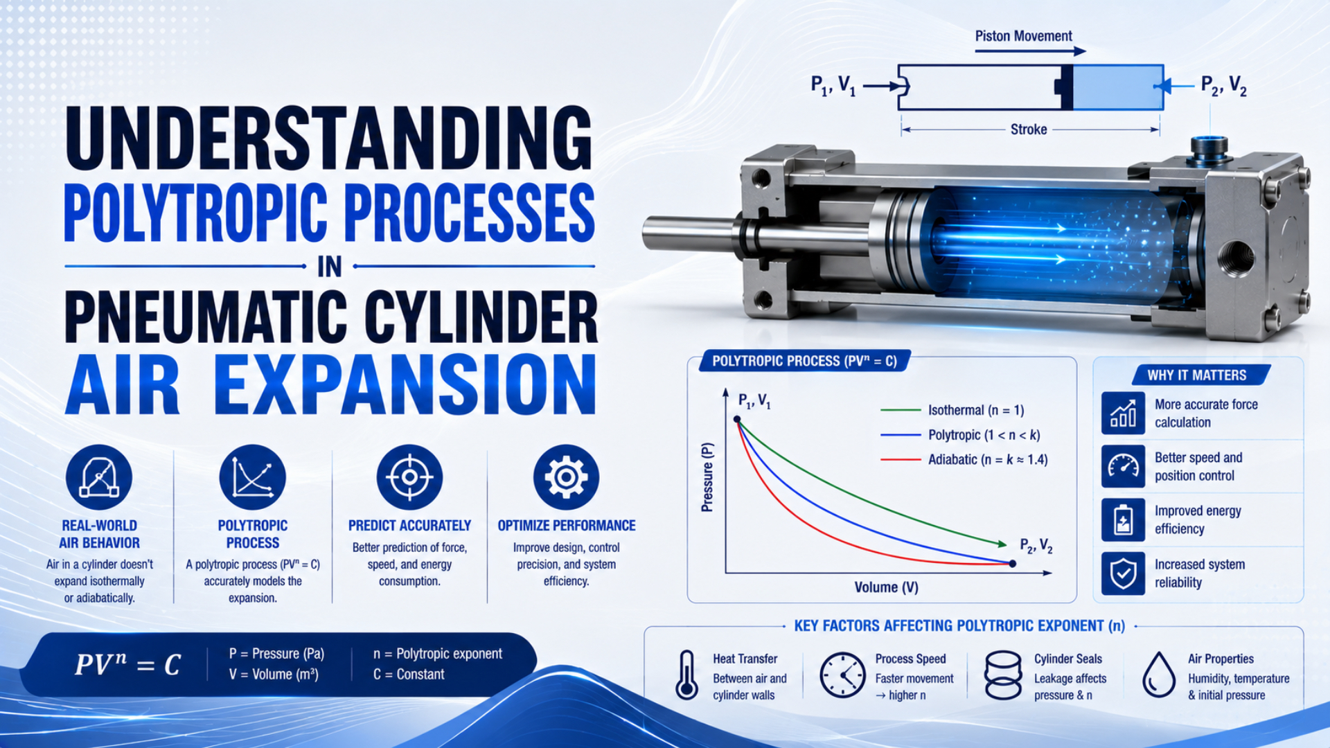
A polytropic process is an idealized path described by $pV^n=C$. It can approximate a fixed mass of trapped air over a defined pressure-volume interval. It does not, by itself, describe a powered cylinder stroke while a valve supplies one chamber and exhausts the other.

That boundary decides which equation belongs in the analysis. A trapped chamber may support a polytropic fit. A valve-connected chamber requires mass flow, heat transfer, changing volume, two chamber pressures, friction, and load. Treating both situations as the same process can produce a precise answer for the wrong physical system.

Key Takeaways

• MIT identifies 4 notable polytropic limits: constant pressure, constant temperature, reversible adiabatic, and constant volume.
• Use absolute pressure and temperature in gas-state equations.
• Fit $n$ only over a defensible closed-mass interval; use mass and energy balances while valves pass air.

What Is a Polytropic Process?

MIT OpenCourseWare identifies 4 notable cases within the polytropic family: $n=0$ for constant pressure, $n=1$ for constant temperature, $n=\gamma$ for reversible adiabatic behavior, and a very large exponent for nearly constant volume. The exponent defines a modeled path, not a permanent property of a cylinder (MIT OpenCourseWare, 2022).

For a fixed gas mass following one polytropic path:

Here, $p$ is absolute pressure, $V$ is the gas volume, $n$ is the fitted or assumed polytropic exponent, and $C$ is constant over the selected path. The word “selected” matters. A real pressure-volume trace may need different exponents during compression, expansion, dwell, or successive portions of a cycle.

Isothermal behavior means temperature remains constant, giving $n=1$ for an ideal gas of fixed mass. Reversible adiabatic behavior means no heat crosses the boundary and no entropy is generated, giving $n=\gamma$. Near room temperature, dry air is commonly approximated with $\gamma\approx1.4$, but that value is not a universal fitted exponent for working pneumatic hardware.

A measured exponent between 1 and 1.4 can indicate a path between isothermal and reversible adiabatic limits under a suitable closed-mass model. It can also be an average hiding time-dependent heat transfer. Values outside that interval aren’t automatically impossible; they may reflect heat-flow direction, leakage, mass exchange, incorrect dead volume, sensor lag, spatial gradients, or a poor single-exponent fit.

The exponent should be written with its boundary and interval, such as “trapped cap-end chamber, 20% to 70% stroke, expansion fit.” Writing only “$n=1.2$” removes the information needed to decide whether another engineer can reuse it.

Where Does pV^n Apply in a Pneumatic Cylinder?

In a double-acting-cylinder experiment, pressure sensors were placed 5 cm from the chambers and synchronized with displacement measurements. The study modeled chamber pressure using flow, heat-transfer factors, dead volume, and piston motion. That setup shows why a polytropic relation needs a deliberately isolated interval rather than an entire valve-driven stroke (Experimental Techniques, 2020).

The closed-mass approximation is most defensible when the gas being modeled cannot cross the chosen boundary during the interval. Examples include:

Cylinder situation	Is gas mass approximately fixed?	Can $pV^n=C$ be useful?	Main limitation
Both ports blocked after pressure equalizes	Yes, if leakage is negligible	Yes, for small motion or a defined compression/expansion interval	Seal leakage, valve leakage, heat transfer, dead volume
Pneumatic cushion after its exhaust path is effectively restricted	Sometimes	Possibly, over the isolated portion	Cushion needle flow and leakage may keep it open
External load compresses a trapped chamber	Yes, approximately	Yes, for gas-spring stiffness and pressure prediction	Friction and wall heat transfer change the path
Supply valve fills the extending chamber	No	No, not as a complete chamber model	Air mass enters while volume and temperature change
Exhaust valve vents the retracting chamber	No	No, not as a complete chamber model	Air mass leaves through a restriction, often with choked flow

The valve state must be known. A three-position valve with a closed center can trap both chambers during hold, while an exhaust-center valve does not. Check actual spool overlap, leakage, pilot behavior, and any external check valves before calling the chamber closed.

Dead volume belongs inside $V$. Include the end clearance, cushion recess, port cavity, fitting, pressure-sensor passage, and any tube volume that remains on the trapped side of the closed boundary. Omitting it causes the calculated volume ratio to be too large near the end of stroke and can distort the fitted exponent.

For trapped-air stiffness, the air compressibility and cylinder control guide develops the small-signal spring model. This article stays with thermodynamic path selection and exponent estimation.

Why Does a Powered Cylinder Stroke Need an Open-System Model?

A published pneumatic-actuator model uses 2 chamber pressure equations, one for each side of the piston, and includes chamber mass flow, absolute pressure, changing volume, piston velocity, gas temperature, and the heat-capacity ratio. That is the correct category for a valve-connected powered stroke (Actuators, 2019).

For a chamber treated as a control volume, the mass balance is:

The corresponding lumped energy balance can be written as:

Here, $m$ is chamber gas mass, $u$ is specific internal energy, $\dot{Q}$ is heat entering the gas, $p$ is absolute chamber pressure, $V$ is chamber volume, and $h$ is specific enthalpy carried by the entering or leaving stream. Sign conventions and flow properties must remain consistent throughout the model.

This balance exposes what $pV^n=C$ leaves out. During extension, the cap-end chamber often gains air while its volume increases. The rod-end chamber loses air while its volume decreases. Valve restrictions, tube conductance, exhaust back pressure, piston speed, friction, and load determine both pressure histories.

Pressure force therefore comes from measured or modeled chamber pressures, not from a universal force-drop percentage. For cap-end extension:

The two pressures use the same reference, $A_p$ is piston area, and $A_a$ is rod-side annular area. The polytropic exponent can influence a trapped-gas pressure response, but it doesn’t replace the valve-flow and two-pressure calculation during a powered stroke.

What if speed changes while the assumed exponent stays fixed? Inspect dynamic supply pressure, valve conductance, tube size, meter-out setting, exhaust restriction, load, friction, and cushioning. The guide to choked flow and maximum cylinder speed addresses the mass-flow limit; the meter-out control guide covers exhaust back pressure.

A powered stroke and a blocked-port stiffness test may use the same cylinder yet require different thermodynamic models. The hardware did not change. The valve state changed the system boundary.

How Is the Polytropic Index Calculated Correctly?

NASA’s ideal-gas equation connects 4 state variables: pressure, volume, gas mass, and absolute temperature. NIST defines standard atmospheric pressure as 101,325 Pa. Those references establish two non-negotiable rules for fitting a polytropic path: use absolute pressure, and account for every volume inside the selected gas boundary (NASA; NIST).

The ideal-gas state equation is:

Here, $R$ is the specific gas constant and $T$ is absolute temperature. Gauge pressure cannot be inserted into $pV^n=C$ or a logarithmic pressure ratio. Add local atmospheric pressure to gauge pressure, or use an absolute pressure transducer.

For two states on one fixed-exponent path:

Solving for the exponent gives:

Both pressure values must be positive absolute pressures, and the two volumes must represent the same control boundary. The logarithm base does not matter as long as the numerator and denominator use the same base.

For more than two samples, the log-linear form is more informative:

Plot $\ln p$ against $\ln V$ and fit a line. The slope is $-n$. Report the fitted interval, direction of motion, point count, regression method, residuals, uncertainty, sensor locations, dead-volume estimate, and repeatability. A single slope without residuals can hide curvature or two different regimes.

The associated ideal-gas temperature relation is:

Temperatures must be in kelvins or another absolute scale. This relation inherits every assumption behind the polytropic path. It predicts the modeled bulk-gas endpoint, not the cylinder barrel, seal, valve, or exhaust-silencer surface temperature. The adiabatic cooling guide explains that distinction in detail.

What Does n Change in a Closed or Trapped Chamber?

MIT’s ideal limits set $n=1$ for isothermal behavior and $n=\gamma$ for reversible adiabatic behavior. For the same initial pressure, volume, and expansion ratio, a larger exponent produces a lower final pressure and temperature. It does not automatically prove lower machine efficiency, slower motion, or a fixed percentage of force loss (MIT OpenCourseWare, 2022).

Consider a closed, fixed-mass ideal-air example starting at 700 kPa absolute, 0.25 L, and 293.15 K. Let the gas expand to 0.50 L. The calculated endpoints are:

Assumed path	Exponent	Final pressure	Final gas temperature	Boundary work by the gas
Isothermal limit	1.0	350.0 kPa absolute	293.15 K, or 20.0°C	121.3 J
Illustrative polytropic path	1.2	304.7 kPa absolute	255.20 K, or -17.95°C	113.3 J
Reversible adiabatic approximation	1.4	265.3 kPa absolute	222.17 K, or -50.98°C	105.9 J

For $n\ne1$, ideal boundary work is:

For the isothermal case:

These are model outputs, not cylinder ratings. Real metal transfers heat to or from the gas, seals create friction, chamber pressure may be nonuniform, leakage changes mass, and valves may not remain closed. The ideal temperature is especially easy to misuse as a component temperature.

In a small trapped-chamber perturbation, the exponent also appears in pneumatic stiffness:

The equation uses absolute chamber pressure and total trapped volume. It helps explain why a blocked-port cylinder can feel stiffer near one end of its stroke. It doesn’t predict powered-stroke speed. For a double-acting axis, calculate both chamber contributions as shown in the air compressibility control article.

How Can n Be Estimated From Pressure and Position Data?

The 2020 double-acting-cylinder study repeated each test 45 times and synchronously sampled pressure and displacement every 0.1 ms. Those settings belong to that experiment, not a universal requirement, but they illustrate the need for synchronized traces and repeatability when estimating a thermodynamic path (Experimental Techniques, 2020).

Use this sequence for a trapped-chamber test:

1. Define the boundary. Identify the valve state, trapped-side components, expected leakage paths, and whether any check or cushion valve can pass air.
2. Measure absolute pressure. Locate the transducer close enough to represent the chamber without creating an unsafe installation or an unmodeled line delay.
3. Measure piston position. Convert position to chamber volume using effective piston area, stroke datum, and measured or documented dead volume.
4. Synchronize channels. Pressure and position need a shared time base. Temperature, valve command, load, and supply pressure improve diagnosis.
5. Choose a valid interval. Exclude valve switching, mechanical impact, sensor saturation, end-stop contact, and any region where the chamber is not closed.
6. Fit the log relationship. Regress $\ln p$ against $\ln V$, inspect residuals, and calculate uncertainty rather than relying on two endpoints alone.
7. Repeat in both directions. Compression and expansion can produce different paths because heat-flow direction, seal friction, and leakage differ.
8. Validate prediction. Use the fitted exponent to predict a held-out portion or another cycle under the same declared conditions.

Why not prescribe one sampling rate? Required bandwidth depends on chamber size, valve speed, pressure-transducer dynamics, sensor-line volume, piston speed, and the shortest event being resolved. State the sensor bandwidth, sampling rate, filtering, timing uncertainty, and anti-aliasing method instead of copying a generic kilohertz value.

Measurement Errors That Distort the Fitted Index

The same 2020 study placed its chamber-pressure sensors 5 cm from the cylinder and included inactive end volume and port volume in its pressure equations. Both details matter: a remote sensor can lag the chamber, while omitted dead volume changes the calculated volume ratio and therefore the slope used to estimate $n$ (Experimental Techniques, 2020).

Error source	What it does to the fit	Practical check
Gauge pressure used in logarithms	Distorts ratios, especially near atmospheric pressure	Convert to absolute pressure before processing
Dead volume omitted	Exaggerates volume change near an end cap	Measure or estimate ports, recesses, fittings, and trapped tube
Valve still passing air	Violates the fixed-mass assumption	Record valve command and verify the isolated interval
Seal or valve leakage	Changes chamber mass during the fit	Run a pressure-decay check and define acceptable leakage
Pressure sensor connected through a long small tube	Adds delay and pneumatic filtering	Characterize the sensor line or mount closer where safe
Position and pressure clocks misaligned	Pairs the wrong pressure with each volume	Use synchronized acquisition and verify trigger timing
End-stop impact or cushion transition	Adds a different mechanical and flow regime	Exclude the affected interval or model it separately
Heavy filtering	Makes the trace look linear while shifting phase	Report raw bandwidth, filter type, cutoff, and delay
One exponent fitted across curvature	Hides changing heat transfer or boundary conditions	Plot residuals and compare segmented fits

Temperature measurement has its own limits. A wall-mounted sensor does not directly measure bulk gas temperature. A probe inserted into a small chamber can alter dead volume and flow. Fast gas-temperature measurements are difficult, so pressure-position fitting is often more practical, provided the closed-mass assumption is credible.

Uncertainty should travel through the calculation. Pressure accuracy, position resolution, piston-area tolerance, dead-volume uncertainty, and timing offset all influence the slope. Report confidence bounds or a sensitivity range. More decimal places do not make an exponent more transferable.

Residual shape is often more valuable than the exponent itself. Random residuals support a constant-exponent approximation; systematic curvature tells the engineer that heat transfer, leakage, mass exchange, or the chosen interval is changing the process.

Using the Polytropic Index in Design and Troubleshooting

The 2019 actuator study models chamber filling and discharging from ideal-gas, mass-continuity, and energy-conservation laws rather than assigning one complete-stroke exponent. Use $n$ as a local trapped-gas parameter, an empirical comparison metric, or a reduced-order model input, not as a replacement for valve, friction, and load analysis (Actuators, 2019).

Good uses of a defensible exponent include:

• estimating the pressure response of an isolated chamber over the tested volume range;
• calculating local trapped-air stiffness around a stated operating point;
• comparing compression and expansion paths under controlled conditions;
• checking whether a slower event moved closer to an isothermal limit;
• building a reduced-order model that is validated against independent cycles.

Poor uses include applying one exponent to every cylinder size, assigning efficiency from $n$ alone, predicting complete-stroke force without both chamber pressures, or promising energy savings from a different barrel material. Thermal design, valve sizing, control tuning, and maintenance still require their own evidence.

If force is the buyer’s question, start with the pneumatic cylinder theoretical-force guide and then include dynamic back pressure and friction. If the concern is ideal temperature limits, use the adiabatic-versus-isothermal comparison. Those articles answer different questions from fitting $n$.

No existing calculator directly estimates a polytropic exponent from synchronized pressure and position data. A unit converter can prevent input mistakes, but it cannot validate the boundary. Use the Pressure Converter for units, then add atmospheric pressure where gauge-to-absolute conversion requires it.

A Practical Decision Workflow for Cylinder Thermodynamics

NIST gives 101,325 Pa as one standard atmosphere, while real local atmospheric pressure varies. That reference reinforces the first step in any gas-law workflow: establish an absolute-pressure basis. From there, valve state and mass exchange decide whether a polytropic fit or an open-system model is appropriate (NIST).

Use this decision sequence:

1. Name the question. Are you estimating a closed-chamber endpoint, stiffness, powered-stroke pressure, exhaust cooling, force, or cycle time?
2. Draw the boundary. Mark every surface crossed by mass, heat, and mechanical work.
3. Identify the valve state. Confirm whether the chamber is supplied, exhausted, blocked, or connected through a restriction.
4. Choose the model. Use a polytropic path only for an approximately fixed gas mass; otherwise use transient mass and energy balances.
5. Use absolute variables. Pressure and temperature ratios require absolute scales.
6. Include real volume. Add end clearance, ports, fittings, sensor lines, and trapped tubing.
7. Measure competing effects. Record both chamber pressures, position, supply pressure, valve command, load, and time when the powered stroke matters.
8. Fit and challenge the exponent. Inspect residuals, uncertainty, direction, leakage, and validation performance.
9. Keep claims local. Report the exact hardware, interval, cycle condition, and boundary for every fitted value.

Stop if the fitted result contradicts the observed force direction or pressure trace. A lower exponent predicts a slower pressure decrease during closed expansion from the same initial state. It cannot explain a lower final pressure than a higher-exponent model unless another assumption, boundary, initial condition, or measurement has changed.

Polytropic Process FAQs

MIT identifies 4 special polytropic cases, while pneumatic-actuator research uses separate pressure equations for the 2 cylinder chambers. These 5 FAQs keep that distinction visible: polytropic paths describe selected closed-mass behavior, whereas valve-connected motion needs mass flow, energy, pressure, and mechanical dynamics (MIT; Actuators).

Is the polytropic exponent always between 1.0 and 1.4 for air?

No. Those values are useful isothermal and reversible-adiabatic references for an idealized fixed mass near ordinary conditions. A fitted exponent can fall outside that interval because of heat-flow direction, leakage, mass exchange, incorrect volume, sensor lag, or model mismatch. Report the boundary, interval, residuals, and uncertainty with the value.

Can I use pV^n to predict a complete powered cylinder stroke?

Not by itself. While a directional valve is passing air, chamber mass changes as piston motion changes volume. Predicting pressure requires mass flow, energy, heat transfer, valve behavior, and timing. Complete-stroke force also needs both chamber pressures, effective areas, friction, load, and the chosen sign convention.

Why must pressure be absolute when calculating n?

Gas-state equations measure pressure from absolute vacuum. Gauge pressure subtracts the surrounding atmosphere, so its ratio changes incorrectly as chamber pressure approaches ambient. Convert both states to the same absolute-pressure basis before taking logarithms, and document the atmospheric value or absolute transducer used during the test.

Is a fitted n value a cylinder specification?

Usually not. It is a model result for declared hardware, valve state, direction, pressure-volume interval, temperature history, speed, leakage, and measurement setup. The same cylinder can produce different fitted values during compression and expansion or under different timing. Treat transfer to another machine as a new validation task.

Does a lower polytropic exponent guarantee better efficiency?

No. In a closed expansion with the same initial state and final volume, a lower exponent can produce more ideal boundary work because heat enters the gas. Machine efficiency also includes compressor energy, valve losses, leakage, exhaust back pressure, friction, cycle time, controls, and useful work. The exponent alone cannot rank systems.

Sources and technical references

• MIT OpenCourseWare, Thermodynamics and Climate Change, polytropic process definition and special exponent cases; 2022 edition, retrieved 2026-07-22.
• NASA Glenn Research Center, Equation of State for an Ideal Gas, absolute state variables and ideal-gas relationship; retrieved 2026-07-22.
• Position Control of Pneumatic Actuators Using Three-Mode Discrete-Valued Model Predictive Control, two-chamber pressure dynamics derived from ideal-gas, mass-continuity, and energy relations; Actuators, 2019.
• Experimental Study of Double-Acting Pneumatic Cylinder, synchronized chamber-pressure and displacement measurement, dead-volume treatment, sampling, and repeated trials; Experimental Techniques, 2020.
• NIST, SI Units for Pressure, standard atmosphere and pressure-unit guidance; retrieved 2026-07-22.
• Transient Heat Transfer Model and Verification for Gas Cylinder Expansion, time-dependent heat transfer and empirical polytropic characterization in a piston-cylinder experiment; International Journal of Heat and Mass Transfer, 2016.